• Z-Test Assumptions
• Z-Test for Single Proportion - Formulas
• Continuity Correction for Z-Test
• Confidence Interval for Single Proportion
• Agresti-Coull Adjustment for CI

A z-test for a single proportion examines if a
population proportion is likely to be x. Example: does a proportion of 0.60 (or 60%) of some population have antibodies against Covid-19?

If this is true, a sample proportion may differ somewhat from 0.60. However, a very different sample proportion suggests that our initial claim was wrong.

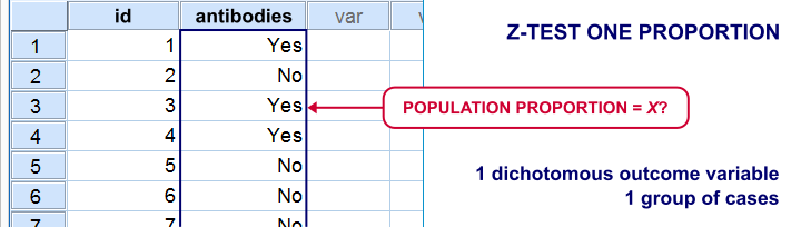
Note that this null hypothesis implies a dichotomous outcome variable: the only 2 possible outcomes are to carry or not to carry such antibodies.

Z-Test Single Proportion - Example

• An epidemiologist believes that 60% of all Dutch adults carry antibodies against Covid-19;
• she samples N = 112 people and administers PCR tests to them;
• 58 people (51.8%) out of 112 people test positive and thus carry antibodies.

Given this outcome, should she still believe that 60% of the entire population carry antibodies? A z-test answers just that but it does require some assumptions.

Z-Test Assumptions

A z-test for a single proportion requires two assumptions:

• independent observations;
• \(n_1 \ge 15\) and \(n_2 \ge 15\): our sample should contain at least some 15 observations for either possible outcome.

Standard textbooks^3,5 often propose \(n_1 \ge 5\) and \(n_2 \ge 5\) but recent studies suggest that these sample sizes are insufficient for accurate test results.²

Z-Test for Single Proportion - Formulas

If sample sizes are sufficient, a sample proportion is approximately normally distributed with

$$\mu_0 = \pi_0$$ and

$$\sigma_0 = SE_0 = \sqrt{\frac{\pi_0(1 - \pi_0)}{N}}$$

where

• \(\pi_0\) denotes the population proportion under the null hypothesis;
• \(SE_0\) denotes the standard error under the null hypothesis;
• \(N\) denotes the total sample size.

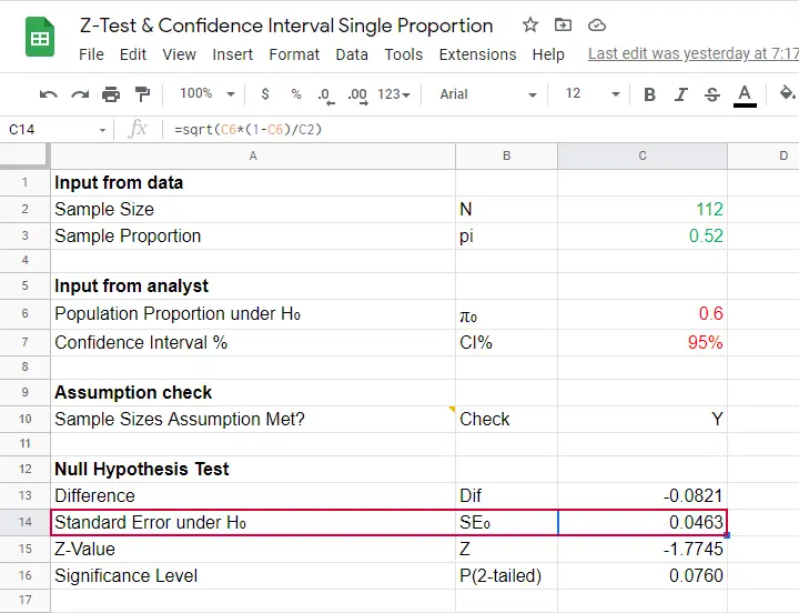
Our example examines if the population proportion \(\pi_0\) is 0.60 using a total sample size of \(N\) = 112 and therefore,

$$SE_0 = \sqrt{\frac{0.60(1 - 0.60)}{112}} = 0.046.$$

Using this outcome, we can standardize our sample proportion \(pi\) into a z-score using

$$Z = \frac{pi - \pi_0}{SE_0}$$

Our sample came up with a proportion \(pi\) of 0.52 because 58 out of 112 people carried Covid-19 antibodies. Therefore,

$$Z = \frac{0.52 - 0.60}{0.046} = -1.77$$

Finally,

$$p(2{\text -}tailed) = 2 \cdot p(z \lt -1.77) = 0.076.$$

This means that if the population proportion really is 0.60, there's a 0.076 (or 7.6%) probability of finding a sample proportion of 0.52 or a more extreme outcome in either direction. Conclusion: we do not reject the null hypothesis that \(\pi_0 = 0.60\) if we test at the usual \(\alpha\) = 0.05 level. All formulas are found in this Googlesheet (read-only), partly shown below.

Continuity Correction for Z-Test

The z-test we just discussed comes up with an approximate significance level. The accuracy of this result can be improved by a simple adjustment:

$$pi_{cc} = \begin{cases} \frac{N \cdot pi \;- \;0.5}{N} \;\;\text{ if } \;\;pi \gt \pi_0\\\\ \frac{N \cdot pi \;+ \;0.5}{N} \;\;\text{ if } \;\;pi \lt \pi_0 \end{cases}$$

This continuity correction simply adds or subtracts 0.5 from the number of successes before converting it into a sample proportion.

For our example, we thus test for

$$pi_{cc} = \frac{112 \cdot 0.52 + 0.5}{N} = 0.522$$

Now, we still compute \(SE_0\) based on \(pi\) but we compute \(Z\) as

$$Z_{cc} = \frac{pi_{cc} - \pi_0}{SE_0} \approx -1.68 $$

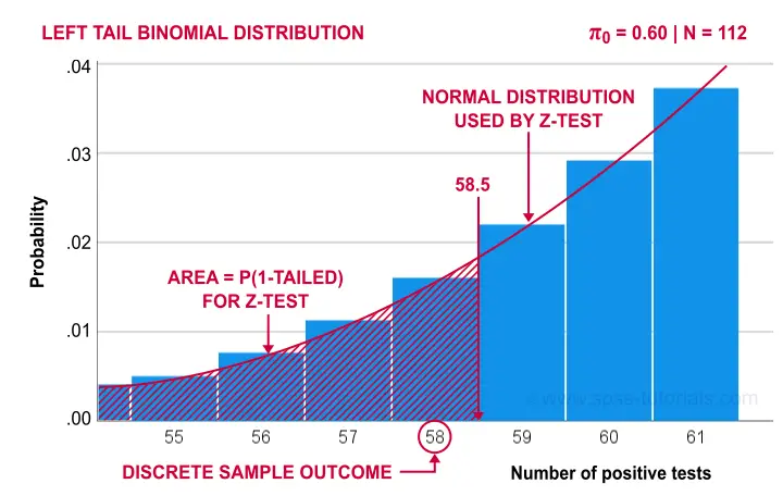
The reason for the continuity correction is that the number of successes strictly follows a binomial distribution. This discrete distribution gives the exact probability for each separate outcome.

When approximating these probabilities with a probability density function -such as the normal distribution- we need to include the entire outcome. This runs from (outcome - 0.5) to (outcome + 0.5) as illustrated below for our example.

Finally, the screenshot below shows the SPSS output for the (un)corrected z-tests.

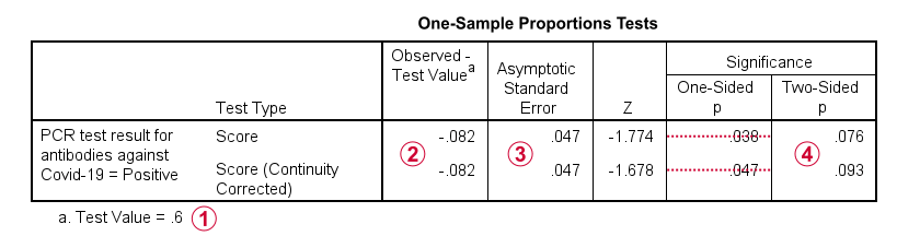
“Test Value” refers to \(\pi_0\), the hypothesized population proportion;

“Observed Test Value” refers to \(pi - \pi_0\);

SPSS reports the wrong standard error for this test;

the z-values and p-values confirm our calculations.

Confidence Interval for Single Proportion

Computing a confidence interval for a proportion uses a different standard error than the corresponding z-test:

$$SE_a = \sqrt{\frac{pi(1 - pi)}{N}}$$

Note that the standard error now uses our sample proportion \(pi\) instead of the hypothesized population proportion \(\pi_0\). Our sample of \(N\) = 112 came up with a proportion of 0.52 and therefore

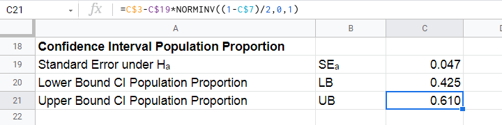
$$SE_a = \sqrt{\frac{0.52(1 - 0.52)}{112}} = 0.047.$$

We can now construct a confidence interval for the population proportion \(\pi\) with

$$CI_{\pi} = pi - SE_a \cdot Z_{1-^{\alpha}_2} \lt \pi \lt pi + SE_a \cdot Z_{1-^{\alpha}_2}$$

For a 95% CI, \(\alpha\) = 0.05. Therefore,

$$Z_{1-^{\alpha}_2} = Z_{.975} \approx 1.96$$

and this results in

$$CI_{\pi} = 0.52 - 0.047 \cdot 1.96 \lt \pi \lt 0.52 + 0.047 \cdot 1.96 = $$

$$CI_{\pi} = 0.43 \lt \pi \lt 0.61$$

This means that the interval [0.43,0.61] has a 95% likelihood of enclosing the population proportion of people carrying antibodies against Covid-19.

The screenshot below shows how to compute this CI in this Googlesheet.

Agresti-Coull Adjustment for CI

We proposed earlier that the aforementioned confidence interval requires that \(n_1 \ge 15\) and \(n_2 \ge 15\). Agresti & Coull (1998)¹ proposed a simple adjustment when this assumption is not met:

• \(n_{1ac} = n_1 + 2\) and
• \(n_{2ac} = n_2 + 2\).

That is, we simply add 2 observations to each group and then proceed as usual. The example presented by the authors involves a sample containing

• \(n_1\) = 0 respondents who own an iPod and
• \(n_2\) = 20 respondents who don't own an iPod.

After adding 2 observations to either group, we simply compute the confidence interval for

• \(n_1\) = 22 respondents don't own an iPod and
• \(n_2\) = 2 respondents do own an iPod.

This initially results in

$$CI_{\pi} = \frac{22}{24} - 0.056 \cdot 1.96 \lt \pi \lt \frac{22}{24} + 0.056 \cdot 1.96 = $$

$$CI_{\pi} = 0.807 \lt \pi \lt 1.027$$

However, since proportions can't be larger than 1, we'll censor this interval to [0.807,1.000].

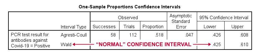
The screenshot below shows the SPSS output for (un)adjusted confidence intervals for our Covid-19 example.

Relation to Other Tests

First off, the z-test for a single proportion without the continuity correction is equivalent to the chi-square goodness-of-fit test: these tests always yield identical p-values.

Second, the z-test for a single proportion with the continuity correction comes very close to the binomial test: for our Covid-19 example,

• p(2-tailed) = .093 for the continuity corrected z-test;
• 2 · p(1-tailed) = .095 for the binomial test.

Note that a binomial test yields an exact p-value for some sample proportion. However, some reasons for not using it are that

• it only yields 1-tailed p-values unless \(\pi\) = 0.50;
• it does not yield any confidence intervals;
• it is computationally intensive for larger sample sizes.

References

1. Agresti, A. & Coull, B.A. (1998). Approximate Is Better than "Exact" for Interval Estimation of Binomial Proportions The American Statistician, 52(2), 119-126.
2. Agresti, A. & Franklin, C. (2014). Statistics. The Art & Science of Learning from Data. Essex: Pearson Education Limited.
3. Van den Brink, W.P. & Koele, P. (1998). Statistiek, deel 2 [Statistics, part 2]. Amsterdam: Boom.
4. Van den Brink, W.P. & Koele, P. (2002). Statistiek, deel 3 [Statistics, part 3]. Amsterdam: Boom.
5. Twisk, J.W.R. (2016). Inleiding in de Toegepaste Biostatistiek [Introduction to Applied Biostatistics]. Houten: Bohn Stafleu van Loghum.