Clustered Bar Chart over Multiple Variables
- Example Data
- VARSTOCASES without VARSTOCASES
- Restructuring the Data
- SPSS Chart Builder - Basic Steps
- Final Result
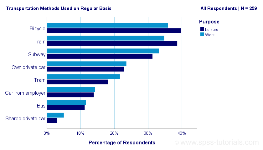
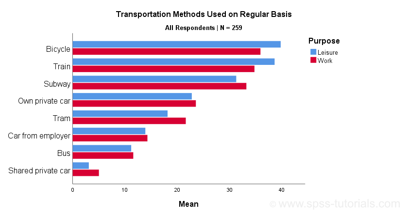
This tutorial shows how to create the clustered bar chart shown below in SPSS. As this requires restructuring our data, we'll first do so with a seriously cool trick.
Example Data
A sample of N = 259 respondents were asked “which means of transportation do you use on a regular basis?” Respondents could select one or more means of transportation for both work and leisure related travelling. The data thus obtained are in transportation.sav, partly shown below.
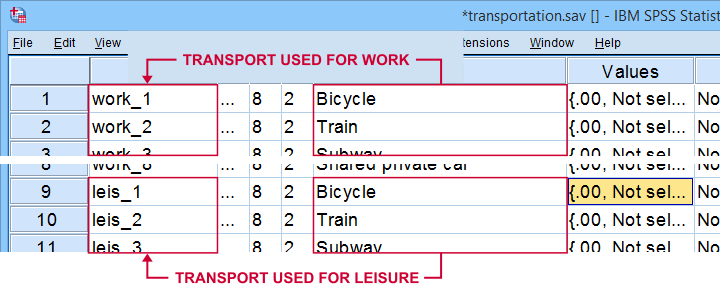
Note that our data consist of 2 sets (work and leisure) of 8 dichotomous variables (transportation options). For creating our chart, we need to stack these 2 sets vertically. The usual way to do so is with VARSTOCASES as illustrated below.
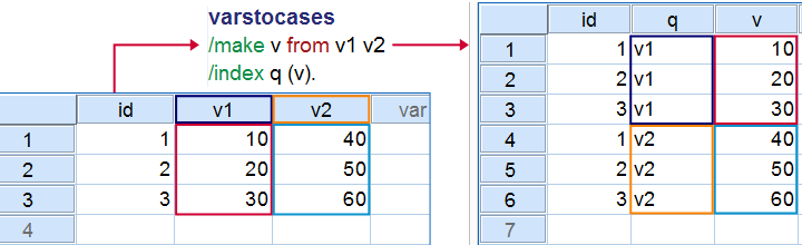
Now, we could use VARSTOCASES for our data but we find this rather tedious for 8 variables. We'll replace it with a trick that creates nicer results and requires less syntax too.
VARSTOCASES without VARSTOCASES
The screenshots below illustrate how to mimic VARSTOCASES without needing its syntax.
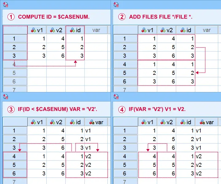
This method saves more effort insofar as you stack more variables: placing the IF command in step  in a DO REPEAT loop does the trick.
Restructuring the Data
Let's now run these steps on transportation.sav with the syntax below. If you're not sure about some command, you can inspect its result in data view if you run EXECUTE right after it.
descriptives all.
*Add id to dataset.
compute id = $casenum.
*Vertically stack dataset onto itself.
add files file */file *.
*Identify copied cases.
compute Purpose = ($casenum > id).
value labels Purpose 0 'Work' 1 'Leisure'.
*Shift values from leisure into work variables.
do repeat #target = work_1 to work_8 / #source = leis_1 to leis_8.
if(purpose) #target = #source.
end repeat.
*Create checktable 2.
means work_1 to work_8 by Purpose.
If everything went right, the 2 checktables will show the exact same information.
Final Data Adjustments
Our data now have the structure required for running our chart. However, a couple of adjustments are still desirable:
- since we want to see percentages instead of proportions, we'll RECODE our 0-1 variables into 0-100;
- next, FORMATS adds percent signs to the recoded values;
- the Chart Builder only computes means over quantitative variables. We'll therefore set all measurement levels to scale;
- we'll remove a couple of variables that have become redundant.
recode work_1 to work_8 (1 = 100).
*Set formats to percentages.
formats work_1 to work_8 (pct8).
*Set measurement levels (needed for SPSS chart builder & Custom Tables).
variable level work_1 to work_8 (scale).
*Remove (now) redundant variables.
add files file */drop leis_1 to id.
SPSS Chart Builder - Basic Steps
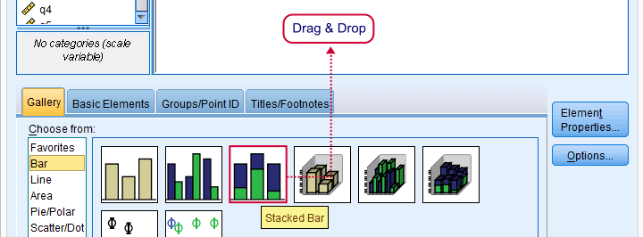
The screenshot below sketches some basic steps that'll result in our chart.
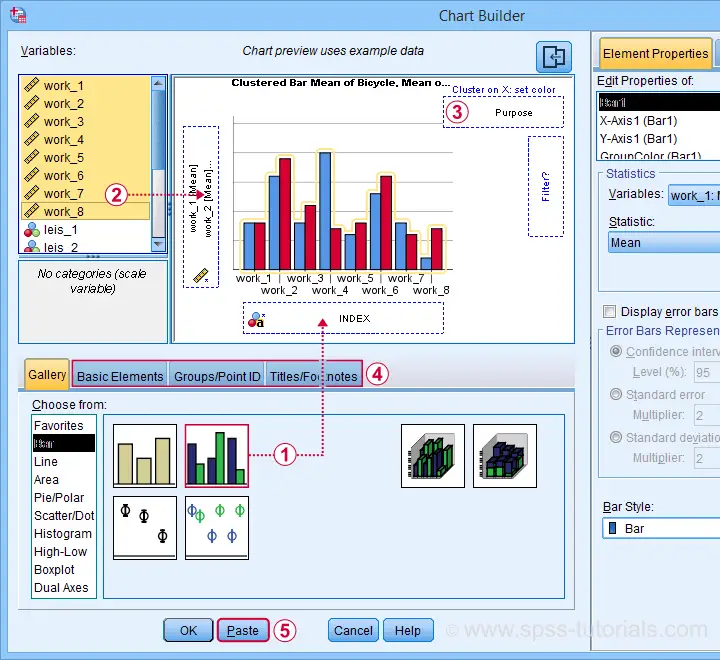
 drag and drop the clustered bar chart onto the canvas;
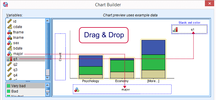
 select, drag and drop all outcome variables in one go into the y-axis box. Click “Ok” in the dialog that pops up;
 drag “Purpose” (leisure or work) into the Color box;
go through these tabs, select “Transpose” and choose some title and subtitle for the chart;
 clicking results in the syntax below.
GGRAPH
/GRAPHDATASET NAME="graphdataset" VARIABLES=MEAN(work_1) MEAN(work_2) MEAN(work_3) MEAN(work_4)
MEAN(work_5) MEAN(work_6) MEAN(work_7) MEAN(work_8) Purpose MISSING=LISTWISE REPORTMISSING=NO
TRANSFORM=VARSTOCASES(SUMMARY="#SUMMARY" INDEX="#INDEX")
/GRAPHSPEC SOURCE=INLINE.
BEGIN GPL
SOURCE: s=userSource(id("graphdataset"))
DATA: SUMMARY=col(source(s), name("#SUMMARY"))
DATA: INDEX=col(source(s), name("#INDEX"), unit.category())
DATA: Purpose=col(source(s), name("Purpose"), unit.category())
COORD: rect(dim(1,2), transpose(), cluster(3,0))
GUIDE: axis(dim(2), label("Mean"))
GUIDE: legend(aesthetic(aesthetic.color.interior), label("Purpose"))
GUIDE: text.title(label("Transportation Methods Used on Regular Basis"))
GUIDE: text.subsubtitle(label("All Respondents | N = 259"))
SCALE: cat(dim(3), reverse(), include("0", "1", "2", "3", "4", "5", "6", "7"))
SCALE: linear(dim(2), include(0))
SCALE: cat(aesthetic(aesthetic.color.interior), reverse(), include("0.00", "1.00"))
SCALE: cat(dim(1), include("0.00", "1.00"))
ELEMENT: interval(position(Purpose*SUMMARY*INDEX), color.interior(Purpose),
shape.interior(shape.square))
END GPL.
Initial Result
Whoomp! There it is. We created the chart we were looking for. Sadly, it doesn't look too great:
- despite setting all variable formats to PCT4 (percentages with zero decimal places), percent signs are missing from the x-axis;
- the x-axis is labeled “Mean” instead of “Percentage”;
- the chart doesn't show gridlines.
All such issues can be fixed in the Chart Editor which opens if we double-click our chart. A nicer option, though, is developing and applying a chart template. Our final result after doing so is shown below.
Final Result
Right. This tutorial has been pretty heavy on syntax but I hope you got the hang of it. Were you (not) able to recreate our chart? Do you have any other feedback? Please throw us a comment below.
Thanks for reading!
Creating Bar Charts with Means by Category
One of the most common research questions is do different groups have different mean scores on some variable? This question is best answered in 3 steps:
- create a table showing mean scores per group -you'll probably want to include the frequencies and standard deviations as well;
- create a chart showing mean scores per group;
- run some statistical test -ANOVA in this case. However, this is only meaningful if your data are (roughly) a simple random sample from your target population.
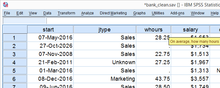
We'll show the first 2 steps using an employee survey whose data are in bank-clean.sav. The screenshot below shows what these data basically look like.
Creating a Means Table
For creating a table showing means per category, we could mess around with
![]()
![]() but its not worth the effort as the syntax is as simple as it gets. So let's just run it and inspect the result.
but its not worth the effort as the syntax is as simple as it gets. So let's just run it and inspect the result.
means q1 by jtype
/cells count mean stddev.
Note that you could easily add more statistics to the CELLS subcommand such as
Result
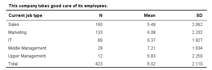
Basically, our table tells us that the mean employee care ratings increase with higher job levels except for “upper management”. A proper descriptives table -always recommended- gives nicely detailed information. However, it's not very visual. So let's now run our chart.
SPSS Bar Chart Menu & Dialogs
As a rule of thumb, I create all charts from
![]() and avoid the Chart Builder whenever I can -which is pretty much always unless I need a stacked bar chart with percentages.
and avoid the Chart Builder whenever I can -which is pretty much always unless I need a stacked bar chart with percentages.
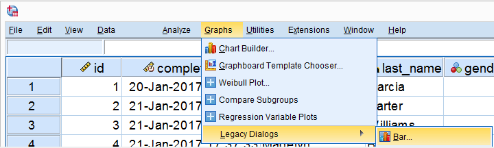
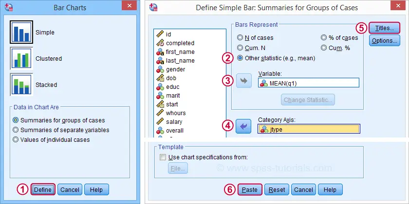
 In the dialog shown below, selecting enables you to
  enter a dependent variable;
Basic Bar Chart Means by Category Syntax
GRAPH
/BAR(SIMPLE)=MEAN(q1) BY jtype
/TITLE='Mean Employee Care Rating by Job Type'
/SUBTITLE='N = 423'.
Result
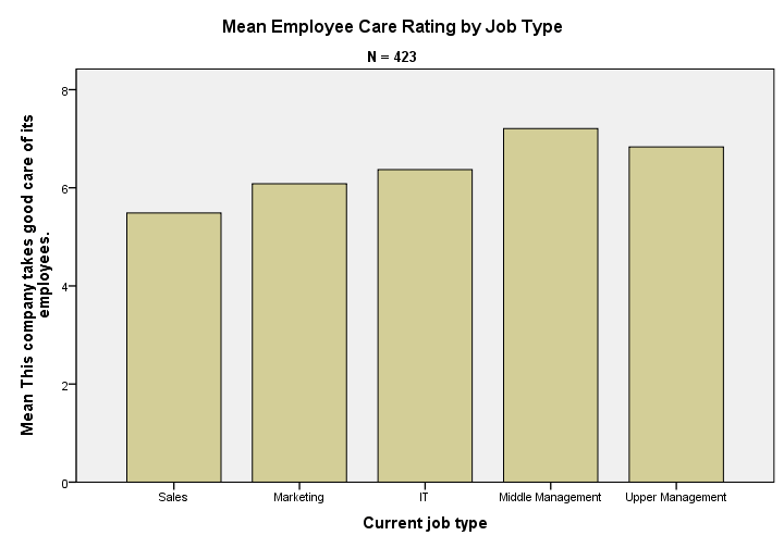
We now have our basic chart but it doesn't look too good.From SPSS version 25 onwards, it will look somewhat better. However, see New Charts in SPSS 25 - How Good Are They Really? Yet. We'll fix this by setting a chart template.
Note that a chart template can also sort this bar chart -for instance by descending means- but we'll skip that for now.
Bar Chart Means by Category Syntax II
set ctemplate "bar-chart-means-trans-720-1.sgt".
*Rerun chart with template set.
GRAPH
/BAR(SIMPLE)=MEAN(q1) BY jtype
/TITLE='Mean Employee Care Rating by Job Type'
/SUBTITLE='N = 423'.
Result
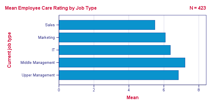
Right, so that's about it. If you need a couple of similar charts, you could copy-paste-edit the last GRAPH command (no need to repeat the other commands). If you need many similar charts, you could loop over the GRAPH command with Python for SPSS.
If you're going to run other types of charts, don't forget to set a different chart template. Or switch if off altogether by running set ctemplate none.
Thanks for reading!
SPSS – Stacked Bar Charts Percentages
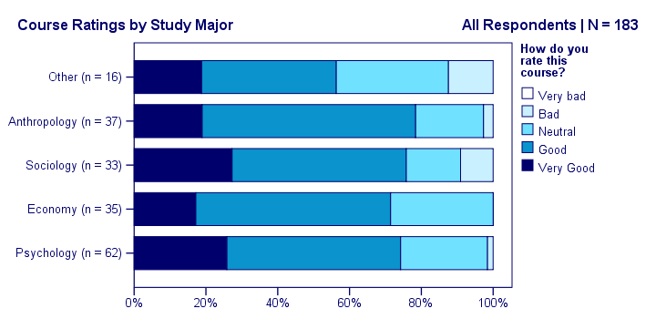
Creating SPSS stacked bar charts with percentages -as shown above- is pretty easy. However, figuring out the right steps may take quite some effort and frustration. This tutorial therefore shows how to do it properly in one go.
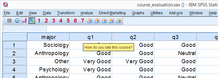
We encourage you to follow along on course_evaluation.sav. Part of these data are shown in the screenshot below.
Example: Course Rating by Study Major
Let's say we'd like to visualize the association between study major (nominal) and overall course rating (ordinal). A table that gives us some insight is a contingency table showing column percentages. We'll create it by running the syntax below.
set tnumbers labels tvars labels.
*Crosstab with column percentages.
crosstabs q1 by major
/cells column.
Result
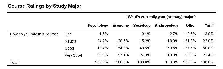
Our course was least popular with students studying some “Other” study major. Can you tell which students like our course most?
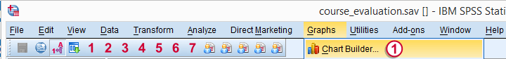
Anyway, it's exactly this table that we'll visualize as a chart. We'll do so by following the next five screenshots.
SPSS Chart Builder Dialogs
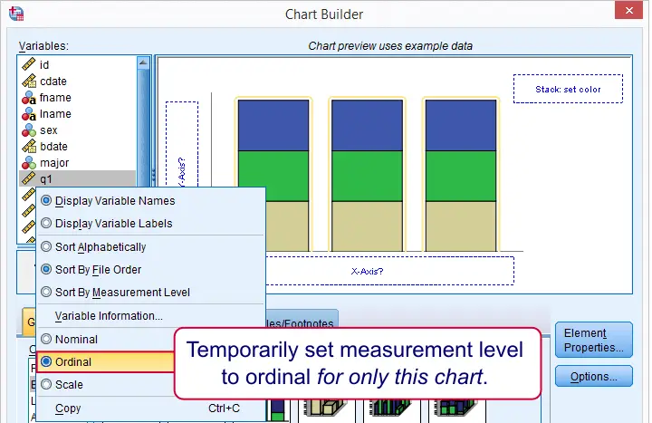
Our stacked bar chart requires setting measurement levels to nominal or ordinal. You could do so before opening the chart builder (possibly preceded by TEMPORARY) or within the chart builder. When using this second option, the chosen measurement levels apply only to the chart you're creating.
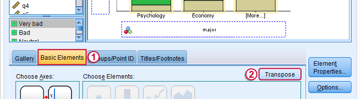
sort of rotates our chart by 90 degrees and thus changes the chart layout from vertical to horizontal. This isn't necessary but the horizontal layout is usually much more suitable for all sorts of bar charts than the default vertical layout.
Two options for transposing charts are 1) in the chart builder as we do now or 2) by applying an SPSS chart template.
 Don't forget to “Apply” here -like I always do.
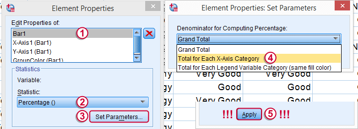
The steps in the screenshot above show the steps for selecting the right percentages for this chart. Don't forget to click whenever changing something in the Element Properties dialog (we forget it all the time).
 And again: “Apply”.
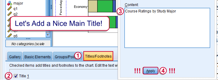
Optionally, set a main title for the chart and it. Clicking results in the syntax below. Let's run it.
SPSS Stacked Bar Chart Syntax
GGRAPH
/GRAPHDATASET NAME="graphdataset" VARIABLES=major COUNT()[name="COUNT"] q1[LEVEL=ORDINAL]
MISSING=LISTWISE REPORTMISSING=NO
/GRAPHSPEC SOURCE=INLINE.
BEGIN GPL
SOURCE: s=userSource(id("graphdataset"))
DATA: major=col(source(s), name("major"), unit.category())
DATA: COUNT=col(source(s), name("COUNT"))
DATA: q1=col(source(s), name("q1"), unit.category())
COORD: rect(dim(1,2), transpose())
GUIDE: axis(dim(1), label("What's currently your (primary) major?"))
GUIDE: axis(dim(2), label("Percent"))
GUIDE: legend(aesthetic(aesthetic.color.interior), label("How do you rate this course?"))
GUIDE: text.title(label("Course Ratings by Study Major"))
SCALE: cat(dim(1), include("1", "2", "3", "4", "5"))
SCALE: linear(dim(2), include(0))
SCALE: cat(aesthetic(aesthetic.color.interior), include("1", "2", "3", "4", "5"))
ELEMENT: interval.stack(position(summary.percent(major*COUNT, base.coordinate(dim(1)))),
color.interior(q1), shape.interior(shape.square))
END GPL.
Unstyled Stacked Bar Chart
First, note that “Very bad” appears in our legend even though it's not present in our data. By default, the Chart Builder includes all values for which value labels are present regardless whether they are present in the data. This can be very annoying: any categories you excluded with FILTER now reappear in your chart.
Second, our chart looks terrible (however, see New Charts in SPSS 25 - How Good Are They Really?). However, a chart template is a great way to fix that. The end result is shown below.
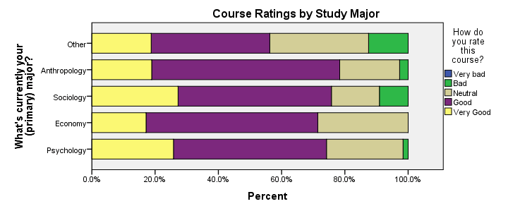
Styled Stacked Bar Chart
Unfortunately, our chart doesn't show any association at all -a bit of an anticlimax after all the work. But I hope you'll have more luck with your charts!
Thanks for reading!
SPSS Bar Charts Tutorial
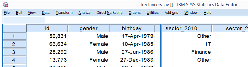
One of the best known charts is a simple bar chart containing frequencies or percentages. The easiest way to run it in SPSS is the FREQUENCIES command. This tutorial walks you through some options. We'll use freelancers.sav throughout, part of which is shown below.
Option 1: FREQUENCIES
In most cases, a simple FREQUENCIES command is our best option because it takes multiple variables in one go. Its syntax -shown below- is so simple that just typing it is probably faster than messing around with the menu.
frequencies sector_2010 to sector_2014
/format notable
/barchart.
Result - Basic
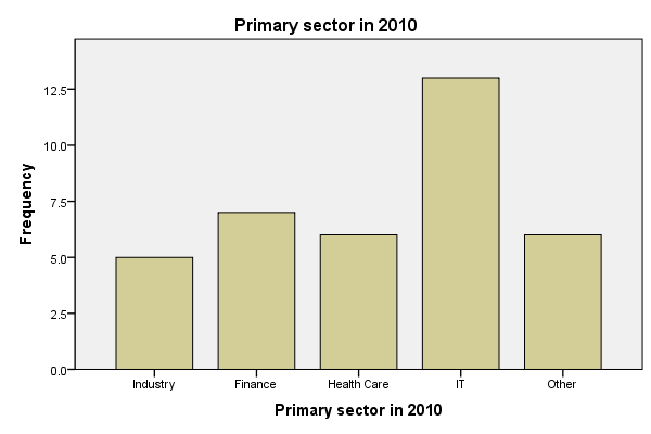
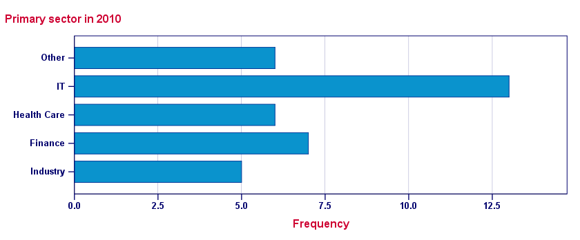
Unsurprisingly, we created the desired bar charts but -like most SPSS charts- they look awful. A great way to fix that is using an SPSS chart template. Just one template is sufficient for having pretty bar charts for once and for all.
A chart template can also transpose (“put on its side”) our chart, which works much better for bar charts than SPSS’ default orientation. One of the charts that resulted from the template we built is shown below.
Result - Chart Template
Sorting Categories and Percentages
A nice -albeit little known- option is sorting the categories. If we transpose our chart, we can sort our bars by descending frequency by specifying /FORMAT NOTABLE AFREQ (use DFREQ for untransposed charts).
Second, we can have percentages instead of frequencies by using /BARCHART PERCENT as shown in the syntax below.
Sorted Bar Charts with Percentages Syntax
frequencies sector_2010
/format notable afreq
/barchart percent.
Result
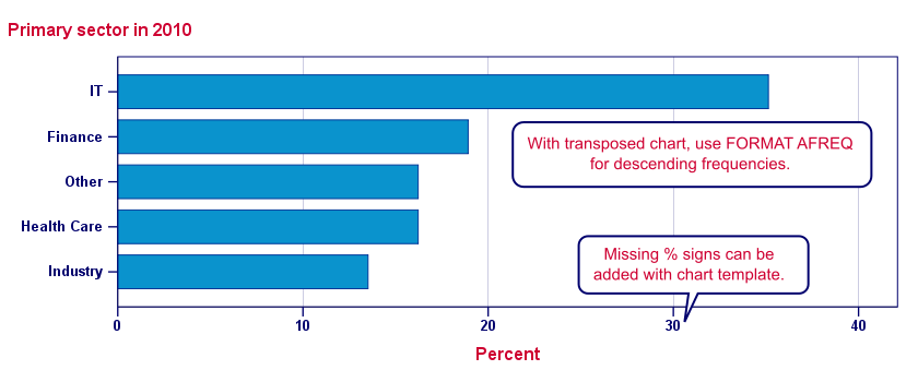
Note: the %-sign is missing from our chart but we can fix this by modifying our chart template.
Option 2: GRAPH
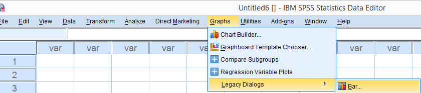
When we run bar charts with FREQUENCIES, the variable labels of the variables involved are used as chart titles. If we want custom titles instead, we're perhaps better off by using GRAPH.Alternatively, set the desired chart titles as new variable labels. Preceding this with TEMPORARY restores the old labels. Since its syntax is a bit more difficult, we'll generate it from the menu as shown below.
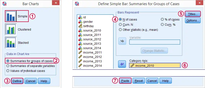
Resulting Syntax
GRAPH
/BAR(SIMPLE)=PCT BY sector_2010
/TITLE='All Respondents | n = 40'.
Note: unfortunately, GRAPH takes only one variable at the time. However, we can remove the line breaks from the syntax and copy-paste-edit it a couple of times for a handful of variables. For running charts or tables over many variables, see SPSS with Python - Looping over Scatterplots.
Second, GRAPH does not allow us to sort our categories but a chart template can fix that.
SPSS Bar Charts - Chart Sizes
One issue with all SPSS charts is that their sizes are fixed in pixels. However, a bar chart for many categories needs more space than a chart for few categories. In fact, categories may disappear altogether if they don't fit into the chart anymore. SPSS does not offer a solution for this other than “stretching” each chart manually in the output viewer. For a better solution, see SPSS - Set Chart Sizes Tool.
With respect to the layout of reports, we prefer having the heights (rather than the widths) of our charts depend on the amount of content they contain. This is yet another good reason for always transposing our bar charts.
Conclusion
In most cases, typing a simple FREQUENCIES command is by far the best option for creating bar charts. GRAPH as pasted from ![]() is a reasonable option too.
is a reasonable option too.
As with most charts, ![]() is better avoided since it's way more complicated and results in the exact same chart as the aforementioned options.
is better avoided since it's way more complicated and results in the exact same chart as the aforementioned options.
Bar Charts - FREQUENCIES Versus GRAPH
The table below quickly summarizes the differences between the two options we discussed in this tutorial.
| Feature | FREQUENCIES | GRAPH |
|---|---|---|
| Multiple variables | Yes | No |
| Category sorting | Yes | Only with chart template |
| Percent sign | Only with chart template | Yes |
| Custom title | No | Yes |