How to Convert String Variables into Numeric Ones?
Introduction & Practice Data File
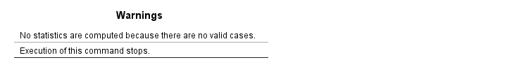
Converting an SPSS string variable into a numeric one is simple. However, there's a huge pitfall that few people are aware of: string values that can't be converted into numbers result in system missing values without SPSS throwing any error or warning.
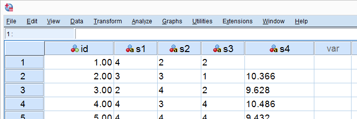
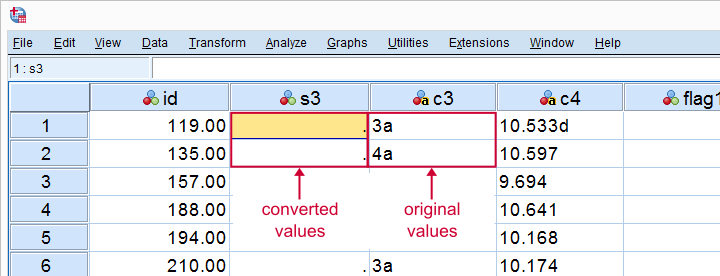
This can mess up your data without you being aware of it. Don't believe me? I'll demonstrate the problem -and the solution- on convert-strings.sav, part of which is shown below.
SPSS Strings to Numeric - Wrong Way
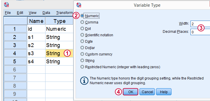
First off, you can convert a string into a numeric variable in variable view as shown below.
Now, I never use this method myself because
- I can't apply it to many variables at once, so it may take way more effort than necessary;
- it doesn't generate any syntax: there's no button and nothing's appended to my journal file;
- it can mess up the data. However, there's remedies for that.
So What's the Problem?
Well, let's do it rather than read about it. We'll
- set empty cells as user missing values for s3;
- convert s3 to numeric in variable view;
- run descriptives on the result.
missing values s3 ('').
*Inspect frequency table for s3.
frequencies s3.
*Now manually convert s3 to numeric under variable view.
*Inspect result.
descriptives s3.
*N = 444 instead of 459. That is, 15 values failed to convert and we've no clue why.
Result
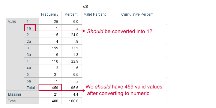
Note that some values in our string variable have been flagged with “a”. We probably want these to be converted into numbers. We have 459 valid values (non empty cells).

After converting our variable to numeric, we ran some descriptives. Note that we only have N = 444. Apparently, 15 values failed to convert -probably not what we want. And we usually won't notice this problem because we don't get any warning or error.
Conversion Failures - Simplest Solution
Right, so how can we perform the conversion safely? Well, we just
- inspected frequency tables: how many non empty values do we have before the conversion?
- converted our variable(s) to numeric;
- inspected N in a descriptive statistics after the conversion. If N is lower than the number of non empty string values (frequencies before conversion), then something may be wrong.
In our first example, the frequency table already suggested we must remove the “a” from all values before converting the variable. We'll do just that in a minute.
Although safe, I still think this method is too much work, especially for multiple variables. Let's speed things up by using some handy syntax.
SPSS - String to Numeric with Syntax
The fastest way to convert string variables into numeric ones is with the ALTER TYPE command.This requires SPSS version 16 or over. For SPSS 15 or below, use the NUMBER function. It allows us to convert many variables with a single line of syntax.
The syntax below converts all string variables in one go. We then check a descriptives table. If we don't have any system missing values, we're done.
SPSS ALTER TYPE Example
*Convert all variables in one go.
alter type s1 to s3 (f1) s4 (f6.3).
*Inspect descriptives.
descriptives s1 to s4.
Note: using alter type s1 to s4 (f1). will also work but the decimal places for s4 won't be visible. This is why we set the correct f format: f6.3 means 6 characters including the decimal separator and 3 decimal places as in 12.345. Which is the format of our string values.
Result

Since we've 480 cases in our data, we're done for s1. However, the other 3 variables contain system missings so we need to find out why. Since we can't undo the operation, let's close our data without saving and reopen it.
Solution 2: Copy String Variables Before Conversion
Things now become a bit more technical. However, readers who struggle their way through will learn a very efficient solution that works for many other situations too. We'll basically
- copy all string variables;
- convert all string variables;
- compare the original to the converted variables.
Precisely, we'll flag non empty string values that are system missing after the conversion. As these are at least suspicious, we'll call those conversion failures. This may sound daunting but it's perfectly doable if we use the right combination of commands. Those are mainly STRING, RECODE, DO REPEAT and IF.
Copy and Convert Several String Variables
*Copy all string variables.
string c1 to c4 (a7).
recode s1 to s4 (else = copy) into c1 to c4.
*Convert variables to numeric.
alter type s1 to s3 (f1) s4 (f6.3).
*For each variable, flag conversion failures: cases where converted value is system missing but original value is not empty.
do repeat #conv = s1 to s4 / #ori = c1 to c4 / #flags = flag1 to flag4.
if(sysmis(#conv) and #ori <> '') #flags = 1.
end repeat.
*If N > 0, conversion failures occurred for some variable.
descriptives flag1 to flag4.
Result
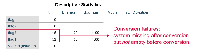
Only flag3 and flag4 contain some conversion failures. We can visually inspect what's the problem by moving these cases to the top of our dataset.
sort cases by flag3 (d).
*Some values flagged with 'a'.
sort cases by flag4 (d).
*Some values flagged with 'a' through 'e'.
Result
Remove Illegal Characters, Copy and Convert
Some values are flagged with letters “a” through “e”, which is why they fail to convert. We'll now fix the problem. First, we close our data without saving and reopen it. We then rerun our previous syntax but remove these letters before the conversion.
Syntax
*Copy all stringvars.
string c1 to c4 (a7).
recode s1 to s4 (else = copy) into c1 to c4.
*Remove 'a' from s3.
compute s3 = replace(s3,'a','').
*Remove 'a' through 'e' from s4.
do repeat #char = 'a' 'b' 'c' 'd' 'e'.
compute s4 = replace(s4,#char,'').
end repeat.
*Try and convert variable again.
alter type s1 to s3 (f1) s4 (f6.3).
*Flag conversion failures again.
do repeat #conv = s1 to s4 / #ori = c1 to c4 / #flags = flag1 to flag4.
if(sysmis(#conv) and #ori <> '') #flags = 1.
end repeat.
*Inspect if conversion succeeded.
descriptives flag1 to flag4.
*N = 0 for all flag variables so we're done.
*Delete copied and flag variables.
delete variables c1 to flag4.
Result
All flag variables contain only (system) missings. This means that we no longer have any conversion failures; all variables have been correctly converted. We can now delete all copy and flag variables, save our data and move on.
Thanks for reading!
Normalizing Variable Transformations – 6 Simple Options
- Overview Transformations
- Normalizing - What and Why?
- Normalizing Negative/Zero Values
- Test Data
- Descriptives after Transformations
- Conclusion
Overview Transformations
| TRANSFORMATION | USE IF | LIMITATIONS | SPSS EXAMPLES |
|---|---|---|---|
| Square/Cube Root | Variable shows positive skewness Residuals show positive heteroscedasticity Variable contains frequency counts | Square root only applies to positive values | compute newvar = sqrt(oldvar). compute newvar = oldvar**(1/3). |
| Logarithmic | Distribution is positively skewed | Ln and log10 only apply to positive values | compute newvar = ln(oldvar). compute newvar = lg10(oldvar). |
| Power | Distribution is negatively skewed | (None) | compute newvar = oldvar**3. |
| Inverse | Variable has platykurtic distribution | Can't handle zeroes | compute newvar = 1 / oldvar. |
| Hyperbolic Arcsine | Distribution is positively skewed | (None) | compute newvar = ln(oldvar + sqrt(oldvar**2 + 1)). |
| Arcsine | Variable contains proportions | Can't handle absolute values > 1 | compute newvar = arsin(oldvar). |
Normalizing - What and Why?
“Normalizing” means transforming a variable in order to
make it more normally distributed.
Many statistical procedures require a normality assumption: variables must be normally distributed in some population. Some options for evaluating if this holds are
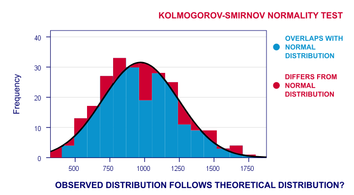
- inspecting histograms;
- inspecting if skewness and (excess) kurtosis are close to zero;
- running a Shapiro-Wilk test and/or a Kolmogorov-Smirnov test.
For reasonable sample sizes (say, N ≥ 25), violating the normality assumption is often no problem: due to the central limit theorem, many statistical tests still produce accurate results in this case. So why would you normalize any variables in the first place? First off, some statistics -notably means, standard deviations and correlations- have been argued to be technically correct but still somewhat misleading for highly non-normal variables.
Second, we also encounter normalizing transformations in multiple regression analysis for
- meeting the assumption of normally distributed regression residuals;
- reducing heteroscedasticity and;
- reducing curvilinearity between the dependent variable and one or many predictors.
Normalizing Negative/Zero Values
Some transformations in our overview don't apply to negative and/or zero values. If such values are present in your data, you've 2 main options:
- transform only non-negative and/or non-zero values;
- add a constant to all values such that their minimum is 0, 1 or some other positive value.
The first option may result in many missing data points and may thus seriously bias your results. Alternatively, adding a constant that adjusts a variable's minimum to 1 is done with
$$Pos_x = Var_x - Min_x + 1$$
This may look like a nice solution but keep in mind that a minimum of 1 is completely arbitrary: you could just as well choose, 0.1, 10, 25 or any other positive number. And that's a real problem because the constant you choose may affect the shape of a variable's distribution after some normalizing transformation. This inevitably induces some arbitrariness into the normalized variables that you'll eventually analyze and report.
Test Data
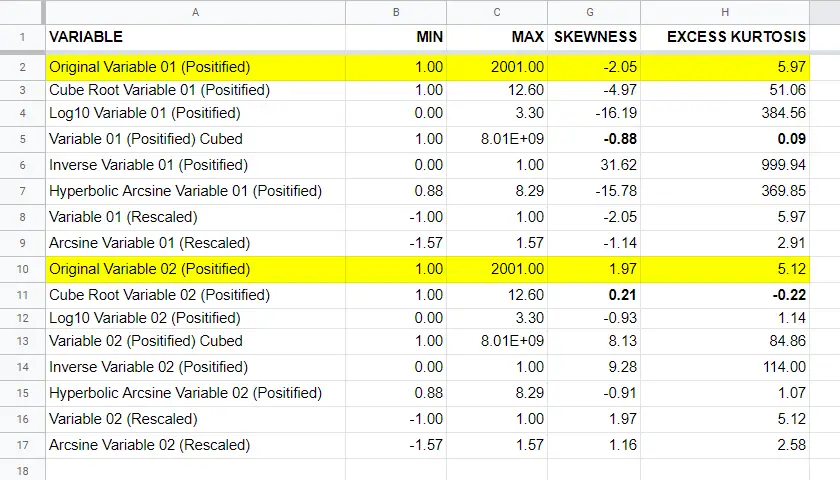
We tried out all transformations in our overview on 2 variables with N = 1,000:
- var01 has strong negative skewness and runs from -1,000 to +1,000;
- var02 has strong positive skewness and also runs from -1,000 to +1,000;
These data are available from this Googlesheet (read-only), partly shown below.
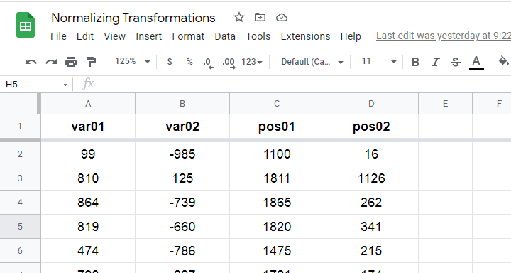
SPSS users may download the exact same data as normalizing-transformations.sav.
Since some transformations don't apply to negative and/or zero values, we “positified” both variables: we added a constant to them such that their minima were both 1, resulting in pos01 and pos02.
Although some transformations could be applied to the original variables, the “normalizing” effects looked very disappointing. We therefore decided to limit this discussion to only our positified variables.
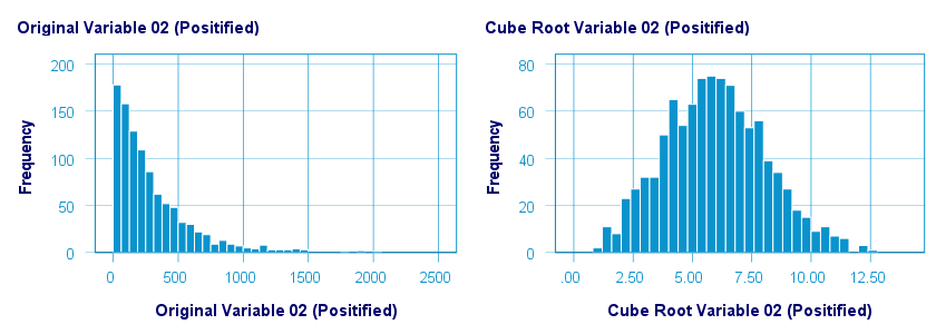
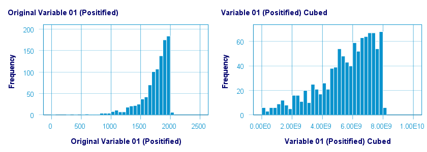
Square/Cube Root Transformation
A cube root transformation did a great job in normalizing our positively skewed variable as shown below.
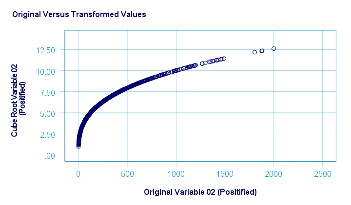
The scatterplot below shows the original versus transformed values.
SPSS refuses to compute cube roots for negative numbers. The syntax below, however, includes a simple workaround for this problem.
compute curt01 = pos01**(1/3).
compute curt02 = pos02**(1/3).
*NOTE: IF VARIABLE MAY CONTAIN NEGATIVE VALUES, USE.
*if(pos01 >= 0) curt01 = pos01**(1/3).
*if(pos01 < 0) curt01 = -abs(pos01)**(1/3).
*HISTOGRAMS.
frequencies curt01 curt02
/format notable
/histogram.
*SCATTERPLOTS.
graph/scatter pos01 with curt01.
graph/scatter pos02 with curt02.
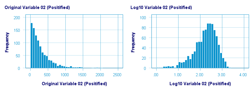
Logarithmic Transformation
A base 10 logarithmic transformation did a decent job in normalizing var02 but not var01. Some results are shown below.
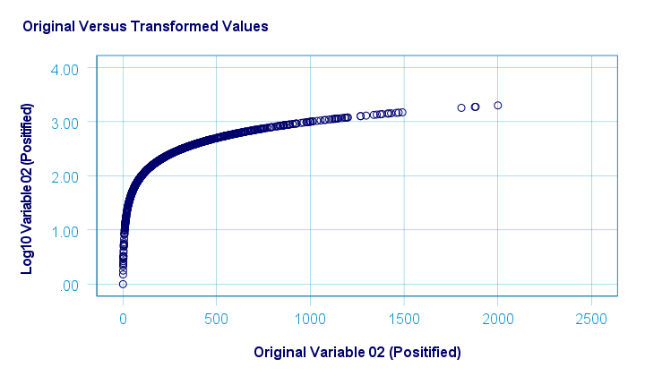
The scatterplot below visualizes the original versus transformed values.
SPSS users can replicate these results from the syntax below.
compute log01 = lg10(pos01).
compute log02 = lg10(pos02).
*HISTOGRAMS.
frequencies log01 log02
/format notable
/histogram.
*SCATTERPLOTS.
graph/scatter pos01 with log01.
graph/scatter pos02 with log02.
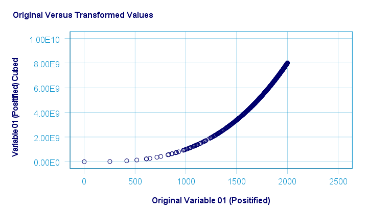
Power Transformation
A third power (or cube) transformation was one of the few transformations that had some normalizing effect on our left skewed variable as shown below.
The scatterplot below shows the original versus transformed values for this transformation.
These results can be replicated from the syntax below.
compute cub01 = pos01**3.
compute cub02 = pos02**3.
*HISTOGRAMS.
frequencies cub01 cub02
/format notable
/histogram.
*SCATTERS.
graph/scatter pos01 with cub01.
graph/scatter pos02 with cub02.
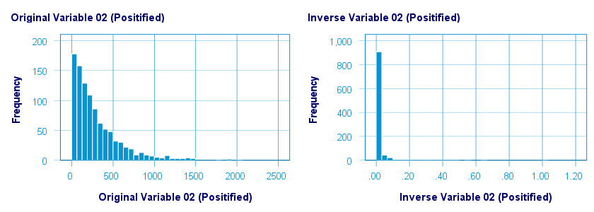
Inverse Transformation
The inverse transformation did a disastrous job with regard to normalizing both variables. The histograms below visualize the distribution for pos02 before and after the transformation.
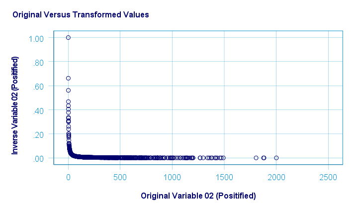
The scatterplot below shows the original versus transformed values. The reason for the extreme pattern in this chart is setting an arbitrary minimum of 1 for this variable as discussed under normalizing negative values.
SPSS users can use the syntax below for replicating these results.
compute inv01 = 1 / pos01.
compute inv02 = 1 / pos02.
*NOTE: IF VARIABLE MAY CONTAIN ZEROES, USE.
*if(pos01 <> 0) inv01 = 1 / pos01.
*HISTOGRAMS.
frequencies inv01 inv02
/format notable
/histogram.
*SCATTERPLOTS.
graph/scatter pos01 with inv01.
graph/scatter pos02 with inv02.
Hyperbolic Arcsine Transformation
As shown below, the hyperbolic arcsine transformation had a reasonably normalizing effect on var02 but not var01.
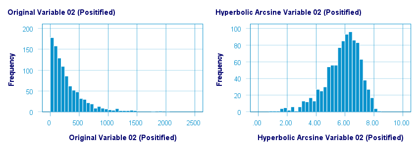
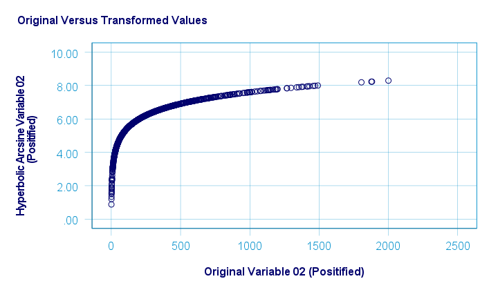
The scatterplot below plots the original versus transformed values.
In Excel and Googlesheets, the hyperbolic arcsine is computed from =ASINH(...) There's no such function in SPSS but a simple workaround is using
$$Asinh_x = ln(Var_x + \sqrt{Var_x^2 + 1})$$
The syntax below does just that.
compute asinh01 = ln(pos01 + sqrt(pos01**2 + 1)).
compute asinh02 = ln(pos02 + sqrt(pos02**2 + 1)).
*HISTOGRAMS.
frequencies asinh01 asinh02
/format notable
/histogram.
*SCATTERS.
graph/scatter pos01 with asinh01.
graph/scatter pos02 with asinh02.
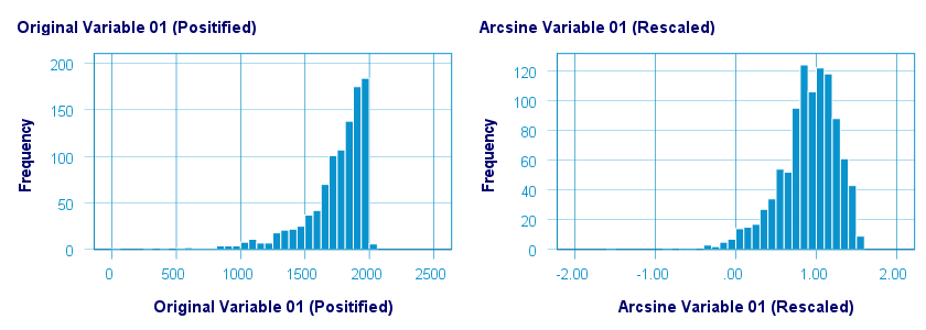
Arcsine Transformation
Before applying the arcsine transformation, we first rescaled both variables to a range of [-1, +1]. After doing so, the arcsine transformation had a slightly normalizing effect on both variables. The figure below shows the result for var01.
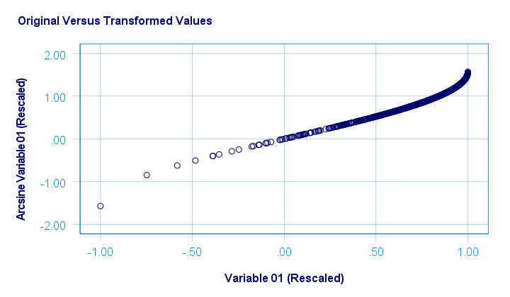
The original versus transformed values are visualized in the scatterplot below.
The rescaling of both variables as well as the actual transformation were done with the SPSS syntax below.
aggregate outfile * mode addvariables
/min01 min02 = min(var01 var02)
/max01 max02 = max(var01 var02).
*RESCALE VARIABLES TO [-1, +1] .
compute trans01 = (var01 - min01)/(max01 - min01)*2 - 1.
compute trans02 = (var02 - min01)/(max01 - min01)*2 - 1.
*ARCSINE TRANSFORMATION.
compute asin01 = arsin(trans01).
compute asin02 = arsin(trans02).
*HISTOGRAMS.
frequencies asin01 asin02
/format notable
/histogram.
*SCATTERS.
graph/scatter trans01 with asin01.
graph/scatter trans02 with asin02.
Descriptives after Transformations
The figure below summarizes some basic descriptive statistics for our original variables before and after all transformations. The entire table is available from this Googlesheet (read-only).
Conclusion
If we only judge by the skewness and kurtosis after each transformation, then for our 2 test variables
- the third power transformation had the strongest normalizing effect on our left skewed variable and
- the cube root transformation worked best for our right skewed variable.
I should add that none of the transformations did a really good job for our left skewed variable, though.
Obviously, these conclusions are based on only 2 test variables. To what extent they generalize to a wider range of data is unclear. But at least we've some idea now.
If you've any remarks or suggestions, please throw us a quick comment below.
Thanks for reading.
SPSS Variable Types and Formats
Understanding SPSS variable types and formats allows you to get things done fast and reliably. Getting a grip on types and formats is not hard if you ignore the very confusing information under variable view. This tutorial will put you on the right track.
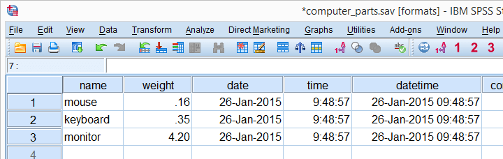
We encourage you to follow along with this tutorial by downloading and opening computer_parts.sav, partly shown below.
SPSS Variable Types
SPSS has 2 variable types:
- Numeric variables contain only numbers and are suitable for numeric calculations such as addition and multiplication.
- String variables may contain letters, numbers and other characters. You can't do calculations on string variables -even if they contain only numbers.
There are no other variable types in SPSS than string and numeric. However, numeric variables have several different formats that are often confused with variable types. We'll see in a minute how variable view puts users on the wrong track here.
The only way to change a string variable to numeric or reversely is ALTER TYPE. However, there's several ways to make a numeric copy of a string variable or reversely. We'll get to those in a minute.
So What's Better: String or Numeric?
The simplest rule of thumb is that
only nominal variables with many categories
should be string variables in SPSS.
Examples are names of people, email addresses, passport numbers and so on. Although such variables can be useful, we don't usually analyze them.
We do sometimes analyze nominal variables with few categories -such as nationality, blood group or profession. If these are string variables, they may or may not cause trouble. For example, the independent variable for ANOVA may or may not be a string variable depending on the exact command you use for it.Precisely, UNIANOVA does and ONEWAY does not accept string variables as factors.
You may get away by leaving such variables as strings. However, copying them into numeric variables makes sure you'll avoid all trouble. A decent way to do so is AUTORECODE. For converting metric string variables -holding just numbers- into numeric variables, see SPSS Convert String to Numeric Variable.
Determining SPSS Variable Types
So how do we know if a variable is string or numeric? In SPSS versions 24 and higher, tiny icons in front of variable names tell us the variable type, format and even measurement level. The icon for “nominal” may contain a tiny “a” which indicates it's a string variable.
For SPSS versions 23 and earlier, we'll inspect our variable view and use the following rule:
- if Type says “String”, you're dealing with a string variable;
- if Type does not say “String”, you're dealing with a numeric variable.
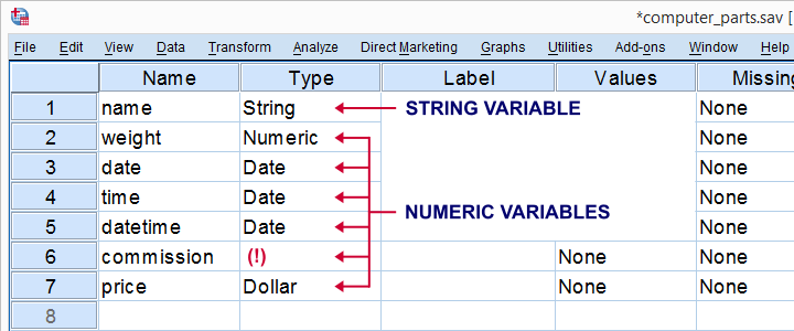
SPSS suggests that “Date” and “Dollar” are variable types as well. However, these are formats, not types. The way they are shown here among the actual variable types (string and numeric) is one of SPSS’ most confusing features.
SPSS Variable Formats - Introduction
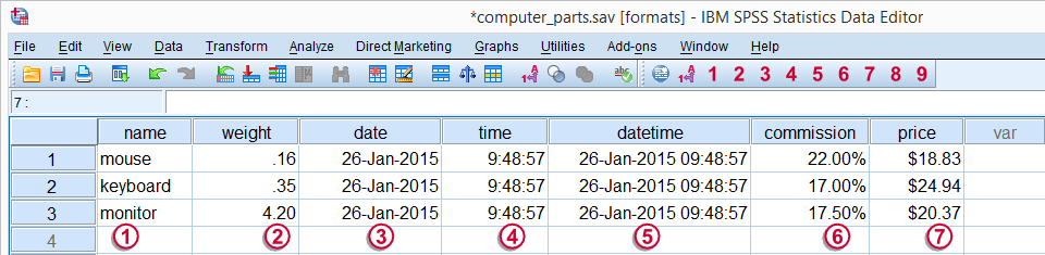
Let's now have a look at the data in data view as shown the screenshot below. We'll briefly describe the kinds of variables we see.
Regarding these data, we stated earlier that
 is a string variable and
 through
  are numeric variables and contain only numbers.
However, values such as “26-jan-2015” sure don't look like numbers, do they? This is because SPSS can display numbers in very different ways. These ways of displaying data values are referred to as variable formats.
Determining SPSS Variable Formats
As we saw earlier, “Type” under variable view shows a confusing mixture of variable types and formats. We'll see the actual formats by running display dictionary. Part of the result is shown by the screenshot below.
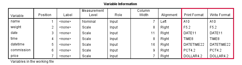
SPSS distinguishes print and write formats but we don't bother about this distinction. SPSS variable formats consist of two parts. One or more letters indicate the format family. Most of them speak to themselves, except for the first two variables:
- A (“Alphanumeric”) is the usual format for string variables;
- F, (“Fortran”) indicates a standard numeric variable.
Formats end with numbers, indicating the number of characters to be shown. If a period is present, the number after the period indicates the number of decimal places to be displayed. The figure below illustrates these points.

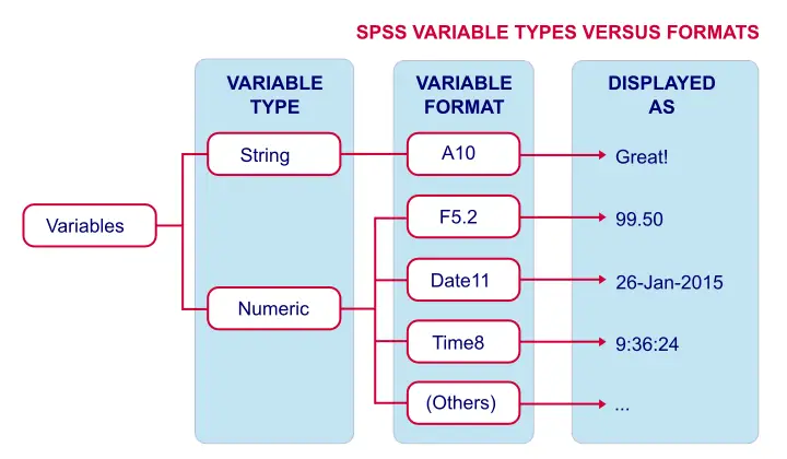
SPSS Common Variable Formats
The figure below now summarizes some common variable types and formats we'll encounter in SPSS.
Setting Variable Formats in SPSS
You can set variable formats for numeric variables with the FORMATS command. For example, formats weight (f4.3). shows weight with 3 decimal places. Doing so affects the output you create: most tables will add an extra decimal place for weight as well. If you'd like to see this for yourself, run the syntax below and compare the 2 resulting tables.
formats weight(f3.2).
descriptives weight.
*Show 3 decimal places for weight and run descriptives.
formats weight(f4.3).
descriptives weight.
*Note that second output table shows more decimal places.
Keep in mind that changing variable formats does not change your data in any way. The actual values are still the exact same numbers. They are merely displayed differently.
Variable Types and Formats - Why Bother?
Basically, “what you see is not what you get” in data view. For example, we see $20.37 but the actual value is just 20.37. So we can identify products costing $20,- or more by running the syntax below:
compute expensive = (price >= 20).
We don't include the dollar sign in our syntax. Although SPSS shows a dollar sign in data view, the actual values are just numbers and these are what the syntax acts upon.
Or let's say we'd like to add 30 days to our date variable. We could do so by running
compute newdate = datesum(date,30,'days').
The resulting values are 13644236937.72. These are the correct numbers but they'll display as readable dates only after running something like
formats newdate (date11).
Another reason for bothering about variable formats is setting decimals places for output tables. For SPSS version 22 onwards, OUTPUT MODIFY does the trick as shown below.
descriptives weight.
*Set 2 decimal places (format = f3.2) for mean and SD (columns 4 and 5).
output modify
/select tables
/tablecells select = [position(4) position(5)] selectdimension = columns format = 'f3.2'.
In a similar vein, CTABLES allows choosing different formats for different statistics in your output.
ctables
/table commission [count 'N' f3 Minimum pct3 Maximum pct3 mean 'Mean' pct4.1 stddev 'SD' pct4.1].
Final Notes
This tutorial was somewhat theoretical but it has a lot of practical consequences. I hope you found it helpful.
Thanks for reading!