Split-Half Reliability in SPSS
- Quick Data Screening
- SPSS Split-Half Reliability Dialogs
- SPSS Split-Half Reliability Output
- Spearman-Brown & Horst Formulas
- Specifying our Test Halves
A psychologist is developing a scale to measure “emotional stability”. She therefore administered her 15 items to a sample of N = 924 students. The data thus obtained are in split-half-reliability.sav, partly shown below.
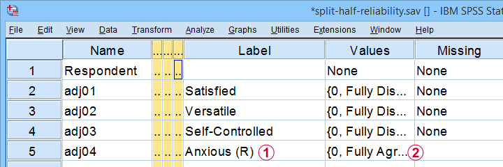
Note that some items indicating emotional instability have been reverse coded. These items  have (R) appended to their variable label and
  their value labels have been adjusted as well.
Now, test reliability is usually examined using Cronbach’s alpha. However, some researchers prefer split-half reliability:
- the items are divided over two test halves;
- the sum scores over the items in each half are computed;
- the Pearson correlation between these 2 sum scores is computed;
- this correlation is adjusted for test length and reported.
So how to find split-half reliability in SPSS? We'll show you in a minute. But let's first make sure we know what's in our data.
Quick Data Screening
A solid way to screen these data is inspecting frequency distributions and their corresponding bar charts. You'll find these under
![]()
![]() but a faster way is to run the SPSS syntax below.
but a faster way is to run the SPSS syntax below.
frequencies adj01 to adj15
/barchart.
Data Screening Output
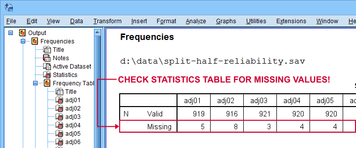
First off, note that the Statistics table indicates that there's some missing values in our variables. Fortunately, they're not too many but they'll have consequences for our analyses nevertheless.
Next up, let's inspect the actual frequency tables. The main question here is whether we should specify any answer categories (such as “No opinion”) as user missing values. Note that these are not present in the data at hand.
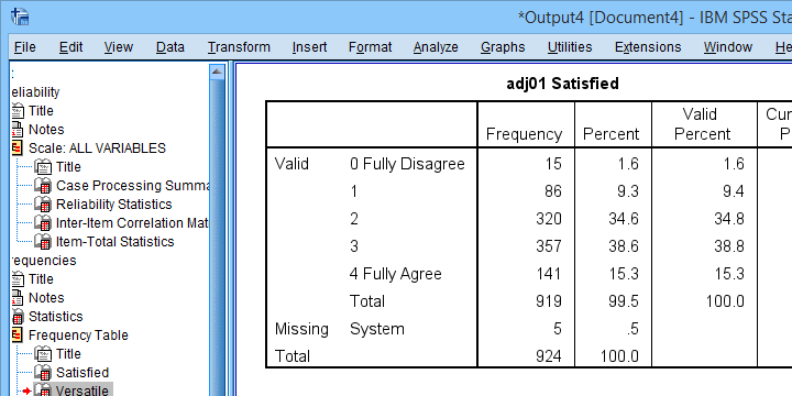
Quick tip: if your tables don't show the actual values (0, 1, ...), then run set tnumbers both tvars both. prior to running your tables as covered in SPSS SET - Quick Tutorial.
Last but not least, scroll through your bar charts like the one shown below.
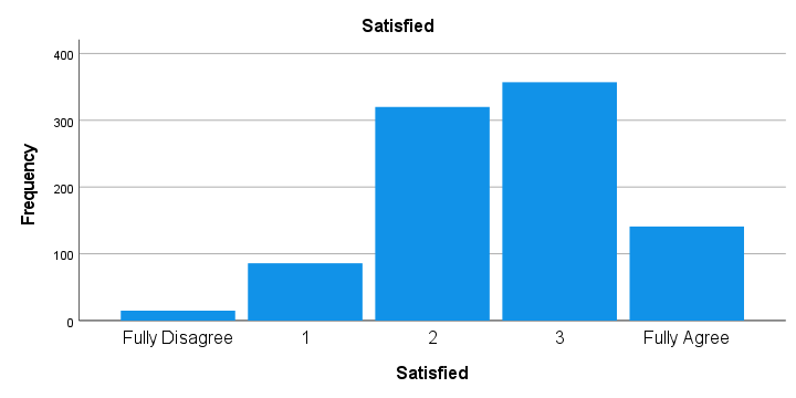
The bar charts for our example data all look perfectly plausible. Most of them have some negative skewness but this makes sense for these data.
So except for a couple of missing values, our data look fine. We can now analyze them with confidence.
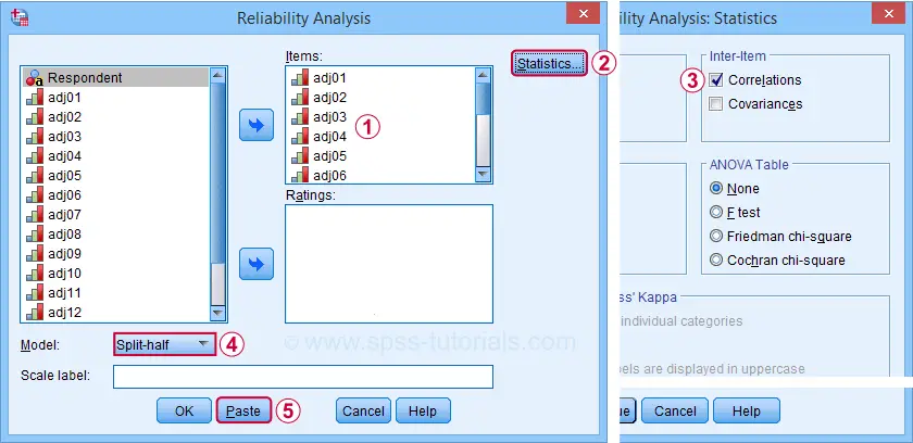
SPSS Split-Half Reliability Dialogs
We'll first navigate to
![]()
![]() and fill out the dialogs as shown below.
and fill out the dialogs as shown below.
Completing these steps results in the syntax below. Let's run it.
RELIABILITY
/VARIABLES=adj01 adj02 adj03 adj04 adj05 adj06 adj07 adj08 adj09 adj10 adj11 adj12 adj13 adj14 adj15
/SCALE('ALL VARIABLES') ALL
/MODEL=SPLIT
/STATISTICS=CORR.
SPSS Split-Half Reliability Output
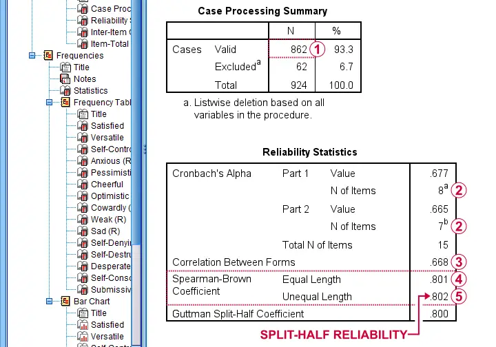
First off, note that this analysis is based on N = 862 out of 924 observations due to missing values.
Next, SPSS defines Part 1 (the first test half) as the first 8 items. As seen in the footnotes, the last 7 items make up Part 2.
 The (unadjusted) correlation between the sum scores over these halves, r = .668.
 Adjusting this correlation using the Spearman-Brown formula results in rsb = .801. We'll explain the what and why for this adjustment in a minute.
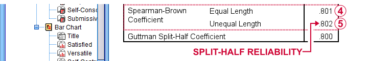
 If our test “halves” have unequal lengths, the more appropriate adjustment is the Horst formula6 which results in rh = .802. This is what we report as our split-half reliability.
Note that we also have the correlation matrix among all items in our output. I recommend you quickly scan it for any negative correlations. These don't make sense among items that measure a single trait. So if you do find them, something may be wrong with your data.
For the data at hand, adj12 (Self-Destructive) has some negative correlations. Although they're probably not statistically significant, this item seems rather poor and had perhaps better be removed from our scale.
Quick Replication of Results
Let's now see if we can replicate some of these results. First off, we'll recompute the correlation between the sum scores of our test halves using the syntax below.
compute first8 = sum.8(adj01 to adj08)./*SUM.8 = COMPUTE SUM ONLY FOR COMPLETE CASES.
compute last7 = sum.7(adj09 to adj15).
correlations first8 last7.
This -indeed- yields r = .668. So why and how should this be adjusted?
Spearman-Brown & Horst Formulas
It is well known that test reliability tends to increase with test length1,7: everything else equal, more items result in higher reliability.
Now, with split-half reliability, we compute the reliability for test halves. And because these are only half as long as the entire test, this greatly attenuates our reliability estimate.
So which correlation would we have found for test halves
having the same length as the entire test?
This can be estimated by the Spearman-Brown formula, which is
$$r_{sb} = \frac{k \cdot r}{1 + (k - 1) \cdot r}$$
where
- \(r_{sb}\) denotes the Spearman-Brown adjusted correlation;
- \(k\) denotes the factor by which the test length increases and;
- \(r\) denotes unadjusted correlation between test halves.
In this formula,
$$k = \frac{number\;of\; items\; in\; new\; test}{number\;of\; items\; in\; old\; test}$$
For our example, the entire test contains 15 items while our halves have an average length of (8 + 7) / 2 = 7.5 items. Therefore, k = 15 / 7.5 = 2.
That is, our test length increases by a factor 2 (note that this is always the case for split-halves reliability).
Now our Spearman-Brown adjusted correlation is
$$r_{sb} = \frac{2 \cdot 0.668}{1 + (2 - 1) \cdot 0.668} = .801$$
which is precisely what SPSS reports. There's one minor issue, though: the Spearman-Brown formula assumes that the test halves have equal lengths.
If this doesn't hold, Warrens6 (2016) argues that the Horst formula should be used instead. In the SPSS output, this is denoted as “Spearman-Brown Coefficient Unequal Length.”
For our example, \(r_h\) = .802 so this is what we report as our split-half reliability.
A minor note here is that the Horst formula simplifies to the Spearman-Brown formula for equal lengths so you can't go wrong by reporting this. Second, Warrens (2016) states that the Horst formula always yields a higher correlation for unequal lengths but the difference tends to be negligible.
Specifying our Test Halves
Now what if we'd like to define our test halves differently? That's fairly simple: for k items, SPSS always uses
- the first k / 2 items as part 1 and all other items as part 2 if k is even;
- the first k / 2 + 0.5 items as part 1 if k is odd.
That is, for 15 items, the first 8 items that you enter are always part 1. All other items are part 2. So if we'd like to use items 1 - 7 as our first half, we simply specify them after items 8 - 15 as shown below.
RELIABILITY
/VARIABLES=adj08 adj09 adj10 adj11 adj12 adj13 adj14 adj15 adj01 adj02 adj03 adj04 adj05 adj06 adj07
/SCALE('ALL VARIABLES') ALL
/MODEL=SPLIT
/STATISTICS=CORR
/SUMMARY=TOTAL.
Right, so that's all folks. I hope you found this tutorial helpful. If you've any questions or remarks, please throw me a comment below.
Thanks for reading!
References
- Drenth, P. & Sijtsma, K. (2015) Testtheorie. Inleiding in de Theorie van de Psychologische Test en zijn Toepassingen [Test theory. Introduction to the theory of the Psychological Test and its Applications]. Houten: Bohn Stafleu van Loghum
- Field, A. (2013). Discovering Statistics with IBM SPSS Statistics. Newbury Park, CA: Sage.
- Howell, D.C. (2002). Statistical Methods for Psychology (5th ed.). Pacific Grove CA: Duxbury.
- Pituch, K.A. & Stevens, J.P. (2016). Applied Multivariate Statistics for the Social Sciences (6th. Edition). New York: Routledge.
- Warner, R.M. (2013). Applied Statistics (2nd. Edition). Thousand Oaks, CA: SAGE.
- Warrens, M.J. (2016). A comparison of reliability coefficients for psychometric tests that consist of two parts. Advances in Data Analysis and Classification, 10(1), 71-84.
- Van den Brink, W.P. & Mellenberg, G.J. (1998). Testleer en testconstructie [Test science and test construction]. Amsterdam: Boom.
How to Compute Means in SPSS?
Introduction & Practice Data File
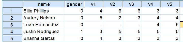
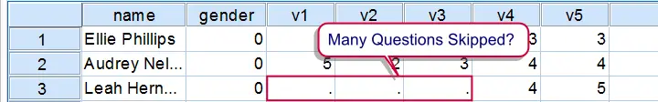
This tutorial shows how to compute means over both variables and cases in a simple but solid way. We encourage you follow along by downloading and opening restaurant.sav, part of which is shown below.
Quick Data Check
Before computing anything whatsoever, we always need to know what's in our data in the first place. Skipping this step often results in ending up with wrong results as we'll see in a minute. Let's first inspect some frequencies by running the syntax below.
set tnumbers both.
*Quick data check.
frequencies v1 to v5.
Result
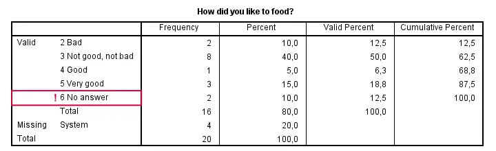
Right, now there's two things we need to ensure before proceeding. Firstly, do all variables have similar coding schemes? For the food rating, higher numbers (4 or 5) reflect more positive attitudes (“Good” and “Very good”) but does this hold for all variables? If we take a quick peek at our 5 tables, we see this holds.
Second, do we have any user missing values? That is, do we want to include all data values in our computations? In this case, we don't. We need to exclude 6 (“No answer”) from all computations. We'll do so with the syntax below.
Setting Missing Values
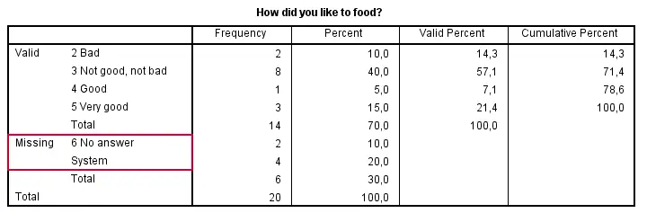
missing values v1 to v5 (6).
*Check again.
frequencies v1 to v5.
Result
Computing Means over Variables
Right, the simplest way for computing means over variables is shown in the syntax below. Note that we can usually specify variable names separated by spaces but for some odd reason we need to use commas in this case.
compute happy1 = mean(v1, v2, v3, v4, v5).
execute.
If our target variables are adjacent in our data, we don't need to spell out all variable names. Instead, we'll enter only the first and last variable names (which can be copy-pasted from variable view into our syntax window) separated by TO.
compute happy2 = mean(v1 to v5).
execute.
Computing Means - Dealing with Missing Values
If we take a good look at our data, we see that some respondents have a lot of missing values on v1 to v5. By default, the mean over v1 to v5 is computed for any case who has at least one none missing value on those variables. If all five values are (system or user) missing, a mean can't be computed so it will be a system missing value as we see in our data.
 It's quite common to exclude cases with many missings from computations. In this case, the easiest option is using the dot operator. For example
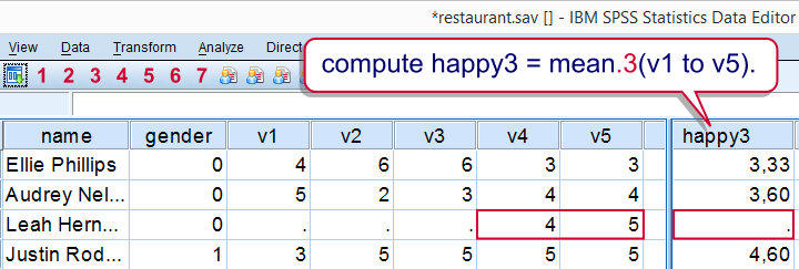
 mean.3(v1 to v5) means “compute means over v1 to v5 but only for cases having at least 3 non missing values on those variables”. Let's try it.
Computing Means - Exclude Cases with Many Missings
compute happy3 = mean.3(v1 to v5).
execute.
Result
A more general way that'll work for more complex computations as well is by using IF as shown below.
if (nvalid (v1 to v5) >= 3) happy4 = mean(v1 to v5).
execute.
SPSS - Compute Means over Cases
So far we computed horizontal means: means over variables for each case separately. Let's now compute vertical means: means over cases for each variable separately. We'll first create output tables with means and we'll then add such means to our data.
Means over all cases are easily obtained with DESCRIPTIVES as in
descriptives v1 v2.
Result
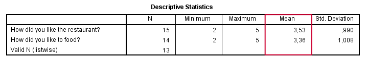
Means for Groups Separately
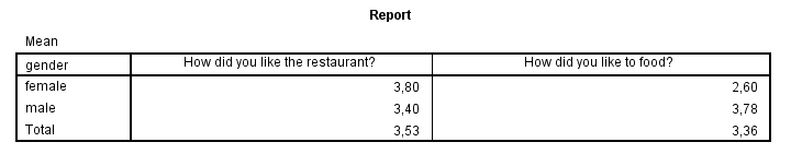
So what if we want means for male and female respondents separately? One option is SPLIT FILE but this is way more work than necessary. A simple MEANS command will do as shown below.
set tnumbers labels.
*Report means for genders separately.
means v1 v2 by gender/cells means.
Result
SPSS - Add Means to Dataset
Finally, you may sometimes want means over cases as new variables in your data. The way to go here is AGGREGATE as shown below.
aggregate outfile * mode addvariables
/mean_1 = mean(v1).
If you'd like means for groups of cases separately, add one or more BREAK variables as shown below. This example also shows how to add means for multiple variables in one go, again by using TO.
aggregate outfile * mode addvariables
/break gender
/mean_2 to mean_5 = mean(v2 to v5).
Result
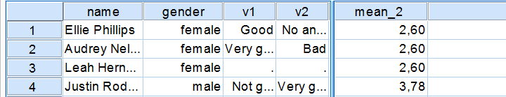
Note that we already saw these means (over v2, for genders separately) in our output after running
means v2 by gender.
Right. That's about all we could think of regarding means in SPSS. If you've any questions or remarks, please feel free to throw in a comment below.
Cronbach’s Alpha in SPSS
Contents
- Cronbach’s Alpha - Quick Definition
- SPSS Cronbach’s Alpha Output
- Increase Cronbach’s Alpha by Removing Items
- Cronbach’s Alpha is Negative
- There are too Few Cases (N = 0) for the Analysis
- APA Reporting Cronbach’s Alpha
Introduction
A psychology faculty wants to examine the reliability of a personality test. They therefore have a sample of N = 90 students fill it out. The data thus gathered are in big-5.sav, partly shown below.
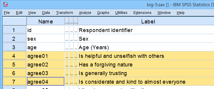
As suggested by the variable names, our test attempts to measure the “big 5” personality traits. For other data files, a factor analysis is often used to find out which variables measure which subscales.
Anyway. Our main research question is: what are the reliabilities for these 5 subscales as indicated by Cronbach’s alpha? But first off: what's Cronbach’s alpha anyway?
Cronbach’s Alpha - Quick Definition
Cronbach’s alpha is the extent to which the sum over 2(+)
variables measures a single underlying trait.
More precisely, Cronbach’s alpha is the proportion of variance of such a sum score that can be accounted for by a single trait. That is, it is the extent to which a sum score reliably measures something and (thus) the extent to which a set of items consistently measure “the same thing”.
Cronbach’s alpha is therefore known as a measure of reliability or internal consistency. The most common rules of thumb for it are that
- Cronbach’s alpha ≥ 0.80 is good and
- Cronbach’s alpha ≈ 0.70 may or may not be just acceptable.
SPSS Reliability Dialogs
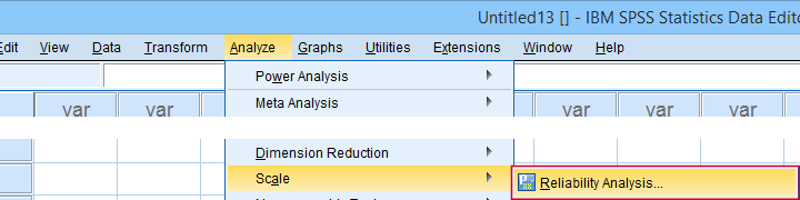
In SPSS, we get Cronbach’s alpha from
![]()
![]() as shown below.
as shown below.
For analyzing the first subscale, agreeableness, we fill out the dialogs as shown below.
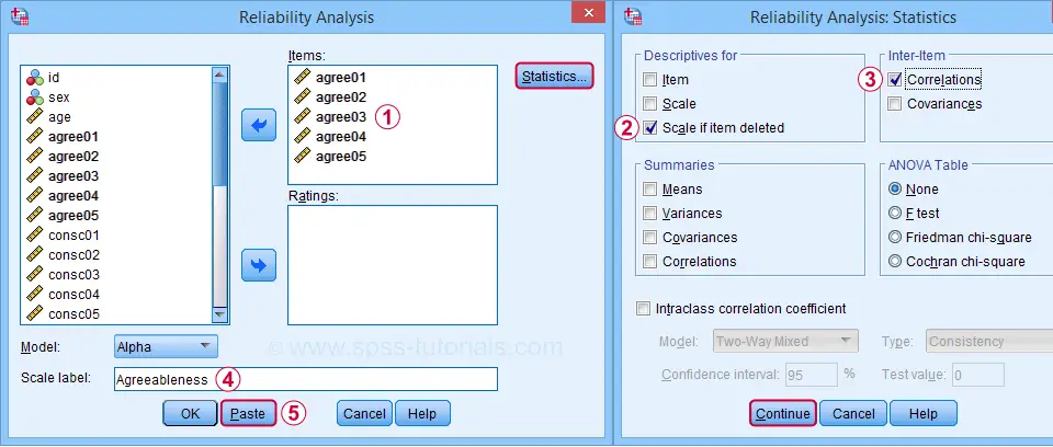
Clicking Paste results in the syntax below. Let's run it.
RELIABILITY
/VARIABLES=agree01 agree02 agree03 agree04 agree05
/SCALE('Agreeableness') ALL
/MODEL=ALPHA
/STATISTICS=CORR
/SUMMARY=TOTAL.
SPSS Cronbach’s Alpha Output I
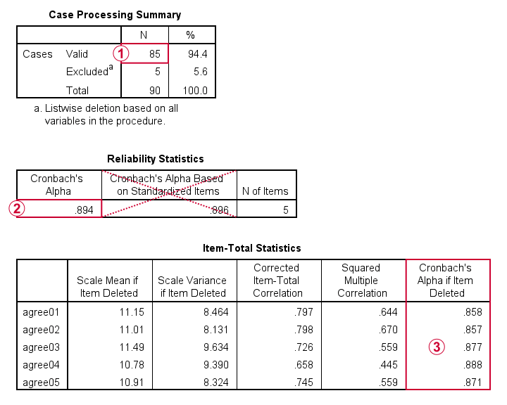
For reliability, SPSS only offers listwise exclusion of missing values: all results are based only on N = 85 cases having zero missing values on our 5 analysis variables or “items”.
Cronbach’s alpha = 0.894. You can usually ignore Cronbach’s Alpha Based on Standardized Items: standardizing variables into z-scores prior to computing scale scores is rarely -if ever- done.
Finally, excluding a variable from a (sub)scale may increase Cronbach’s Alpha. That's not the case in this table: for each item, Cronbach’s Alpha if Item Deleted is lower than the α = 0.894 based on all 5 items.
We'll now run the exact same analysis for our second subscale, conscientiousness. Doing so results in the syntax below.
RELIABILITY
/VARIABLES=consc01 consc02 consc03 consc04 consc05
/SCALE('Conscientiousness') ALL
/MODEL=ALPHA
/STATISTICS=CORR
/SUMMARY=TOTAL.
Increase Cronbach’s Alpha by Removing Items
For the conscientiousness subscale, Cronbach’s alpha = 0.658, which is pretty poor. However, note that Cronbach’s Alpha if Item Deleted = 0.726 for both consc02 and consc04.
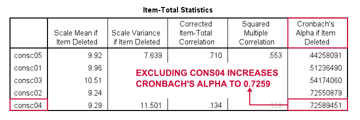
Since removing either item should result in α ≈ 0.726, we're not sure which should be removed first. Two ways to find out are
- increasing the decimal places or (better)
- sorting the table by its last column.
As you probably saw, we already did both with the following OUTPUT MODIFY commands:
output modify
/select tables
/tablecells select = ['Cronbach''s Alpha if Item Deleted'] format = 'f10.8'.
*Sort item-total statistics by Cronbach's alpha if item deleted.
output modify
/select tables
/table sort = collabel('Cronbach''s Alpha if Item Deleted').
It turns out that removing consc04 increases alpha slightly more than consc02. The preferred way for doing so is to simply copy-paste the previous RELIABILITY command, remove consc04 from it and rerun it.
RELIABILITY
/VARIABLES=consc01 consc02 consc03 consc05
/SCALE('Conscientiousness') ALL
/MODEL=ALPHA
/STATISTICS=CORR
/SUMMARY=TOTAL.
After doing so, Cronbach’s alpha = 0.724. It's not exactly the predicted 0.726 because removing consc04 increases the sample size to N = 84. Note that we can increase α even further to 0.814 by removing consc02 as well. The syntax below does just that.
RELIABILITY
/VARIABLES=consc01 consc03 consc05
/SCALE('Conscientiousness') ALL
/MODEL=ALPHA
/STATISTICS=CORR
/SUMMARY=TOTAL.
Note that Cronbach’s alpha = 0.814 if we compute our conscientiousness subscale as the sum or mean over consc01, consc03 and consc05. Since that's fine, we're done with this subscale.
Let's proceed with the next subscale: extraversion. We do so by running the exact same analysis on extra01 to extra05, which results in the syntax below.
RELIABILITY
/VARIABLES=extra01 extra02 extra03 extra04 extra05
/SCALE('Extraversion') ALL
/MODEL=ALPHA
/STATISTICS=CORR
/SUMMARY=TOTAL.
Cronbach’s Alpha is Negative
As shown below, Cronbach’s alpha = -0.663 for the extraversion subscale. This implies that some correlations among items are negative (second table, below).
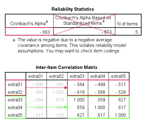
All extraversion items are coded similarly: they have identical value labels so that's not the problem. The problem is that some items measure the opposite of the other items as shown below.
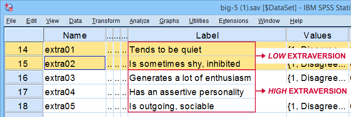
The solution is to simply reverse code such “negative items”: we RECODE these 2 items and adjust their value/variable labels with the syntax below.
RECODE extra01 extra02 (1.0 = 5.0)(2.0 = 4.0)(3.0 = 3.0)(4.0 = 2.0)(5.0 = 1.0).
EXECUTE.
VALUE LABELS
/extra01 5.0 'Disagree strongly' 4.0 'Disagree a little' 3.0 'Neither agree nor disagree' 2.0 'Agree a little' 1.0 'Agree strongly' 6 'No answer'
/extra02 5.0 'Disagree strongly' 4.0 'Disagree a little' 3.0 'Neither agree nor disagree' 2.0 'Agree a little' 1.0 'Agree strongly' 6 'No answer'.
VARIABLE LABELS
extra01 'Tends to be quiet (R)'
extra02 'Is sometimes shy, inhibited (R)'.
Rerunning the exact same reliability analysis as previous now results in Cronbach’s alpha = 0.857 for the extraversion subscale.
So let's proceed with the neuroticism subscale. The syntax below runs our default reliability analysis on neur01 to neur05.
RELIABILITY
/VARIABLES=neur01 neur02 neur03 neur04 neur05
/SCALE('ALL VARIABLES') ALL
/MODEL=ALPHA
/STATISTICS=CORR
/SUMMARY=TOTAL.
There are too Few Cases (N = 0) for the Analysis
Note that our last command doesn't result in any useful tables. We simply get the warning that
There are too few cases (N = 0) for the analysis.
Execution of this command stops.
as shown below.

The 3 most likely causes for this problem are that
- one or more variables contains only missing values;
- an incorrect FILTER filters out all cases in the data;
- missing values are scattered over numerous analysis variables.
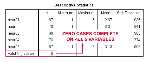
A very quick way to find out is running a minimal DESCRIPTIVES command as in descriptives neur01 to neur05. Upon doing so, we learn that each variable has N ≥ 67 but valid N (listwise) = 0.
So what we really want here, is to use pairwise exclusion of missing values. For some dumb reason, that's not included in SPSS. However, doing it manually isn't as hard as it seems.
Cronbach’s Alpha with Pairwise Exclusion of Missing Values
We'll start off with the formula for Cronbach’s alpha, which is
$$Cronbach’s\;\alpha = \frac{k^2 \overline{S_{xy}}}{\Sigma S^2_x + 2 \Sigma S_{xy}}$$
where
- \(k\) denotes the number of items;
- \(S_{xy}\) denotes the covariance between each pair of different items;
- \(S^2_x\) denotes the sample variance for each item.
Note that a pairwise covariance matrix contains all statistics used by this formula. It is easily obtained via the regression syntax below:
regression
/missing pairwise
/dependent neur01
/method enter neur02 to neur05
/descriptives n cov.
Next, we copy the result into this Googlesheet. Finally, a handful of very simple formulas tell us that α = 0.889.
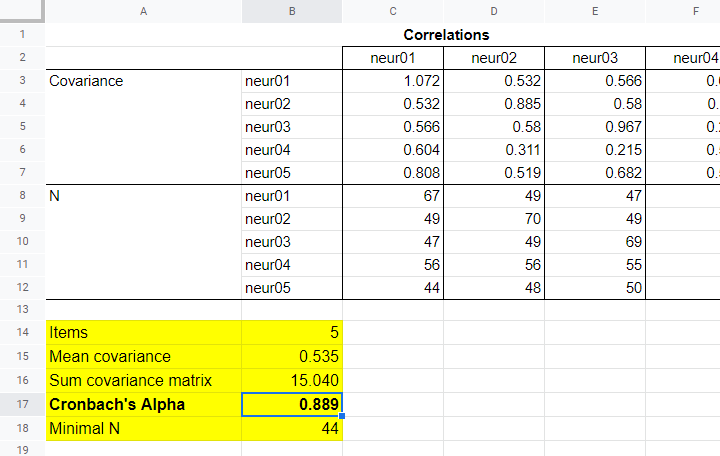
Now, which sample size should we report for this subscale? I propose you follow the conventions for pairwise regression here and report the smallest pairwise N which results in N = 44 for this analysis. Again, note that the formula for finding this minimum over a block of cells is utterly simple.
APA Reporting Cronbach’s Alpha
The table below shows how to report Cronbach’s alpha in APA style for all subscales.
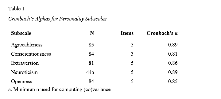
This table contains the actual results from big-5.sav so you can verify that your analyses correspond to mine. The easiest way to create this table is to manually copy-paste your final results into Excel. This makes it easy to adjust things such as decimal places and styling.
Thanks for reading.