SPSS Sign Test for Two Medians – Simple Example

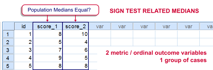
The sign test for two medians evaluates if 2 variables measured on 1 group of cases are likely to have equal population medians.There's also a sign test for comparing one median to a theoretical value. It's really very similar to the test we'll discuss here. Also see SPSS Sign Test for One Median - Simple Example . It can be used on either metric variables or ordinal variables. For comparing means rather than medians, the paired samples t-test and Wilcoxon signed-ranks test are better options.

Adratings Data

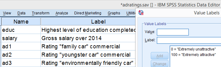
We'll use adratings.sav throughout this tutorial. It holds data on 18 respondents who rated 3 car commercials on attractiveness. Part of its dictionary is shown below.

Descriptive Statistics

Whenever you start working on data, always start with a quick data check and proceed only if your data look plausible. The adratings data look fine so we'll continue with some descriptive statistics. We'll use MEANS for inspecting the medians of our 3 rating variables by running the syntax below.DESCRIPTIVES may seem a more likely option here but -oddly- does not include medians - even though these are clearly “descriptive statistics”.

SPSS Syntax for Inspecting Medians

SPSS Medians Output

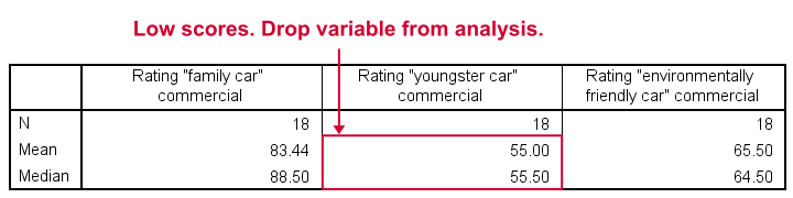
The mean and median ratings for the second commercial (“Youngster Car”) are very low. We'll therefore exclude this variable from further analysis and restrict our focus to the first and third commercials.

Sign Test - Null Hypothesis

For some reason, our marketing manager is only interested in comparing median ratings so our null hypothesis is that the two population medians are equal for our 2 rating variables. We'll examine this by creating a new variable holding signs:

• respondents who rated ad1 < ad3 receive a minus sign;
• respondents who rated ad1 > ad3 get a plus sign.

If our null hypothesis is true, then the plus and minus signs should be roughly distributed 50/50 in our sample. A very different distribution is unlikely under H0 and therefore argues that the population medians probably weren't equal after all.

Running the Sign Test in SPSS

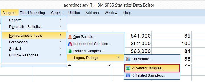
The most straightforward way for running the sign test is outlined by the screenshots below.

The 2 Related samples refer to the two rating variables we're testing. They're related (rather than independent) because they've been measured on the same respondents.

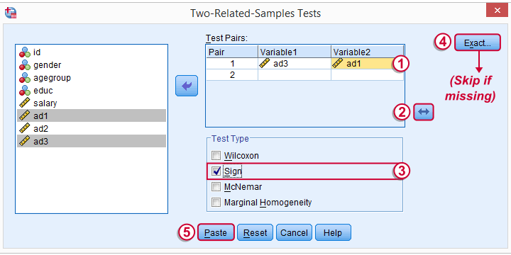
We prefer having the best rated variable in the second slot. We'll do so by reversing the variable order.
Whether your menu includes the Exact button depends on your SPSS license. If it's absent, just skip the step shown below.

SPSS Sign Test Syntax

Completing these steps results in the syntax below (you'll have one extra line if you included the exact test). Let's run it.

Output - Signs Table

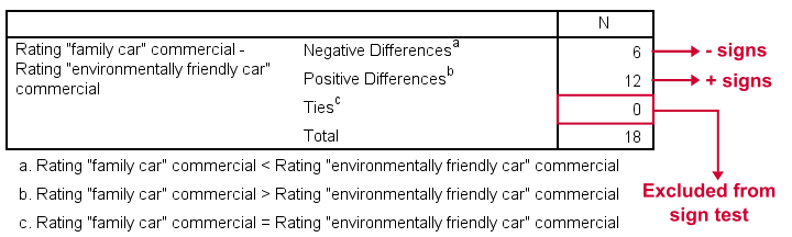
First off, ties (that is: respondents scoring equally on both variables) are excluded from this analysis altogether. This may be an issue with typical Likert scales. The percentage scales of our variables -fortunately- make this much less likely.
Since we've 18 respondents, our null hypothesis suggests that roughly 9 of them should rate ad1 higher than ad3. It turns out this holds for 12 instead of 9 cases. Can we reasonably expect this difference just by random sampling 18 cases from some large population?

Output - Test Statistics Table

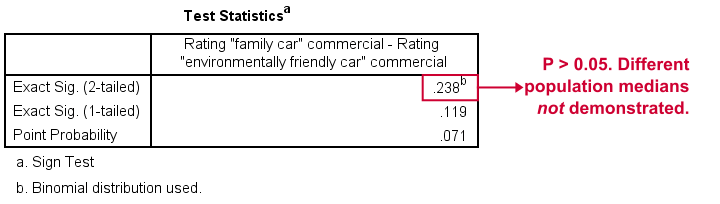
Exact Sig. (2-tailed) refers to our p-value of 0.24. This means there's a 24% chance of finding the observed difference if our null hypothesis is true. Our finding doesn't contradict our hypothesis is equal population medians.
In many cases the output will include “Asymp. Sig. (2-tailed)”, an approximate p-value based on the standard normal distribution.SPSS omits a continuity correction for calculating Z, which (slightly) biases p-values towards zero. It's not included now because our sample size n <= 25.

Reporting Our Sign Test Results

When reporting a sign test, include the entire table showing the signs and (possibly) ties. Although p-values can easily be calculated from it, we'll add something like “a sign test didn't show any difference between the two medians, exact binomial p (2-tailed) = 0.24.”

More on the P-Value

That's basically it. However, for those who are curious, we'll go into a little more detail now. First the p-value. Of our 18 cases, between 0 and 18 could have a plus (that is: rate ad1 higher than ad3). Our null hypothesis dictates that each case has a 0.5 probability of doing so, which is why the number of plusses follows the binomial sampling distribution shown below.

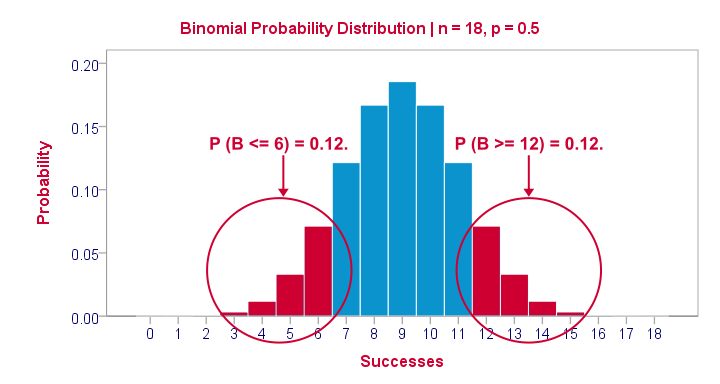
The most likely outcome is 9 plusses with a probability of roughly 0.175: if we'd draw 1,000 random samples instead of 1, we'd expect some 175 of those to result in 9 plusses. Roughly 12% of those samples should result in 6 or fewer plusses or 12 or more plusses. Reporting a 2-tailed p-value takes into account both tails (the areas in red) and thus results in p = 0.24 like we saw in the output.

SPSS Sign Test without a Sign Test

At this point you may see that the sign test is really equivalent to a binomial test on the variable holding our signs. This may come in handy if you want the exact p-value but only have the approximate p-value “Asymp. Sig. (2-tailed)” in your output. Our final syntax example shows how to get it done in 2 different ways.

Workaround for Exact P-Value

SPSS Wilcoxon Signed-Ranks Test – Simple Example

For comparing two metric variables measured on one group of cases, our first choice is the paired-samples t-test. This requires the difference scores to be normally distributed in our population. If this assumption isn't met, we can use Wilcoxon S-R test instead. It can also be used on ordinal variables -although ties may be a real issue for Likert items.
Don't abbreviate “Wilcoxon S-R test” to simply “Wilcoxon test” like SPSS does: there's a second “Wilcoxon test” which is also known as the Mann-Whitney test for two independent samples.

Wilcoxon Signed-Ranks Test - How It Basically Works

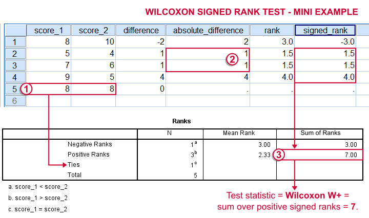
1. For each case calculate the difference between score_1 and score_2. Ties (cases whose two values are equal) are excluded from this test altogether.
2. Calculate the absolute difference for each case.
3. Rank the absolute differences over cases. Use mean ranks for ties (different cases with equal absolute difference scores).
4. Create signed ranks by applying the signs (plus or minus) of the differences to the ranks.
5. Compute the test statistic Wilcoxon W+, which is the sum over positive signed ranks. If score_1 and score_2 really have similar population distributions, then W+ should be neither very small nor very large.
6. Calculate the p-value for W+ from its exact sampling distribution or approximate it by a standard normal distribution.

So much for the theory. We'll now run Wilcoxon S-R test in SPSS on some real world data.

Adratings Data - Brief Description.

A car manufacturer had 18 respondents rate 3 different commercials for one of their cars. They first want to know which commercial is rated best by all respondents. These data -part of which are shown below- are in adratings.sav.

Quick Data Check

Our current focus is limited to the 3 rating variables, ad1 through ad3. Let's first make sure we've an idea what they basically look like before carrying on. We'll inspect their histograms by running the syntax below.

Basic Histograms Syntax

Histograms - Results

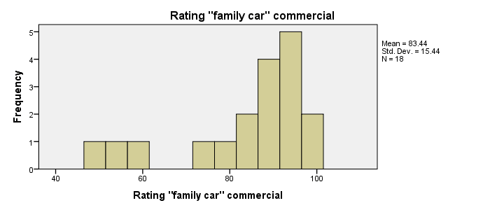
First and foremost, our 3 histograms don't show any weird values or patterns so our data look credible and there's no need for specifying any user missing values.
Let's also take a look at the descriptive statistics in our histograms. Each variable has n = 18 respondents so there aren't any missing values at all. Note that ad2 (the “Youngster car commercial”) has a very low average rating of only 55. It's decided to drop this commercial from the analysis and test if ad1 and ad3 have equal mean ratings.

Difference Scores

Let's now compute and inspect the difference scores between ad1 and ad3 with the syntax below.

Result

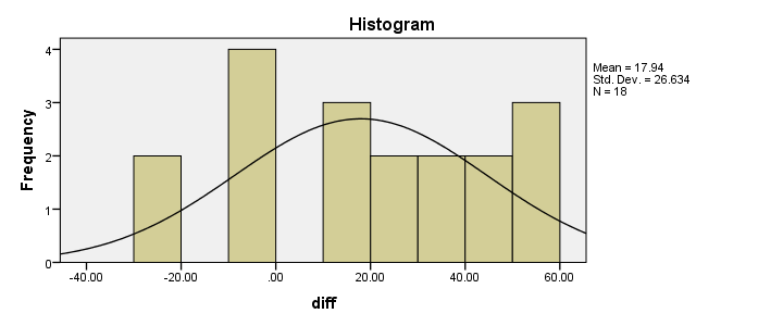
Our first choice for comparing these variables would be a paired samples t-test. This requires the difference scores to be normally distributed in our population but our sample suggests otherwise. This isn't a problem for larger samples sizes (say, n > 25) but we've only 18 respondents in our data.For larger sample sizes, the central limit theorem ensures that the sampling distribution of the mean will be normal, regardless of the population distribution of a variable. Fortunately, Wilcoxon S-R test was developed for precisely this scenario: not meeting the assumptions of a paired-samples t-test. Only now can we really formulate our null hypothesis: the population distributions for ad1 and ad3 are identical. If this is true, then these distributions will be slightly different in a small sample like our data at hand. However, if our sample shows very different distributions, then our hypothesis of equal population distributions will no longer be tenable.

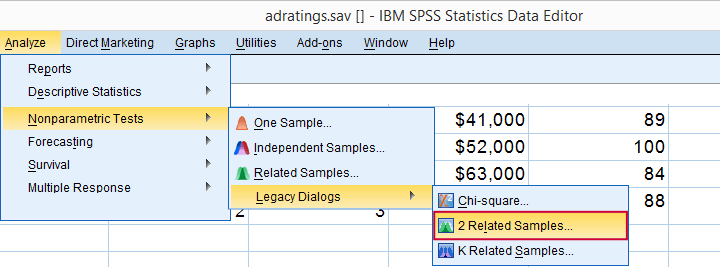
Wilcoxon S-R test in SPSS - Menu

Now that we've a basic idea what our data look like, let's run our test. The screenshots below guide you through.

2 Related Samples refers to comparing 2 variables measured on the same respondents. This is similar to “paired samples” or “within-subjects” effects in repeated measures ANOVA.

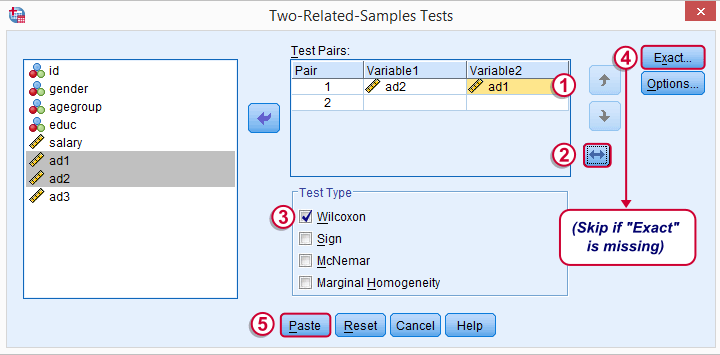
Optionally, reverse the variable order so you have the highest scores (ad1 in our data) under Variable2.
“Wilcoxon” refers to Wilcoxon S-R test here. This is a different test than Wilcoxon independent samples test (also know as Mann-Whitney test).
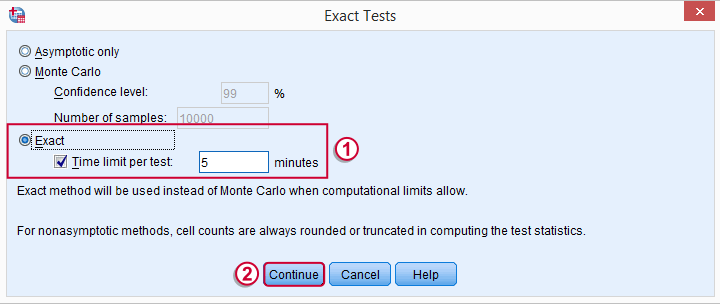
Exact may or may not be present, depending on your SPSS license. If you do have it, we propose you fill it out as below.

Wilcoxon S-R test in SPSS - Syntax

Following these steps results in the syntax below (you'll have one extra line if you requested exact statistics).

Wilcoxon S-R Test - Ranks Table Output

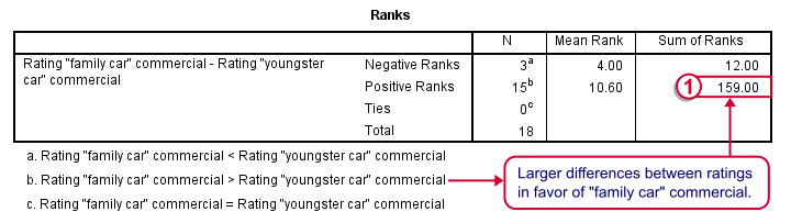
Let's first stare at this table and its footnotes for a minute and decipher what it really says. Right. Now, if ad1 and ad3 have similar population distributions, then the signs (plus and minus) should be distributed roughly evenly over ranks. If you find this hard to grasp -like most people- take another look at this diagram.
This implies that the sum of positive ranks should be close to the sum of negative ranks. This number (159 in our example) is our test statistic and known as Wilcoxon W+.
Our table shows a very different pattern: the sum of positive ranks (indicating that the “Family car” was rated better) is way larger than the sum of negative ranks. Can we still believe our 2 commercials are rated similarly?

Wilcoxon S-R Test - Test Statistics Output

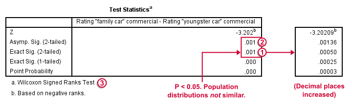
Oddly, our ”Test Statistics“ table includes everything except for our actual test statistic, the aforementioned W+.
We prefer reporting Exact Sig. (2-tailed). Its value of 0.001 means that the probability is roughly 1 in 1,000 of finding the large sample difference we did if our variables really have similar population distributions.
If our output doesn't include the exact p-value, we'll report Asymp. Sig. (2-tailed) instead, which is also 0.001. This approximate p-value is based on the standard normal distribution (hence the “Z” right on top of it).“Asymp” is short for asymptotic. It means that as the sample size approaches infinity, the sampling distribution of W+ becomes identical to a normal distribution. Or more practically: this normal approximation is more accurate for larger sample sizes.
It's comforting to see that both p-values are 0.001. Apparently, the normal approximation is accurate. However, if we increase the decimal places, we see that it's almost three times larger than the exact p-value.A nice tool for doing so is downloadable from Set Decimals for Output Tables Tool.
The reason for having two p-values is that the exact p-value can be computationally heavy, especially for larger sample sizes.

How to Report Wilcoxon Signed-Ranks Test?

The official way for reporting these results is as follows: “A Wilcoxon Signed-Ranks test indicated that the “Family car” commercial (mean rank = 10.6) was rated more favorably than the “Youngster car” commercial (mean rank = 4.0), Z = -3.2, p = 0.001.” We think this guideline is poor for smaller sample sizes. In this case, the Z-approximation may be unnecessary and inaccurate and the exact p-value is to be preferred.

I hope this tutorial has been helpful in understanding and using Wilcoxon Signed-Ranks test in SPSS. Please let me know by leaving a comment below. Thanks!

McNemar Test in SPSS – Comparing 2 Related Proportions

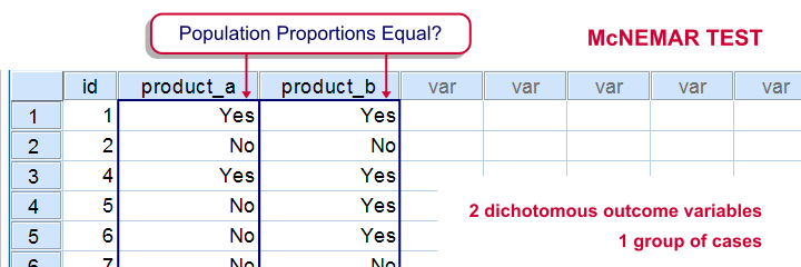
SPSS McNemar test is a procedure for testing if the proportions of two dichotomous variables are equal in some population. The two variables have been measured on the same cases.

SPSS McNemar Test Example

A marketeer wants to know whether two products are equally appealing. He asks 20 participants to try out both products and indicate whether they'd consider buying each products (“yes” or “no”). This results in product_appeal.sav. The proportion of respondents answering “yes, I'd consider buying this” indicates the level of appeal for each of the two products.
The null hypothesis is that both percentages are equal in the population.

1. Quick Data Check

Before jumping into statistical procedures, let's first just take a look at the data. A graph that basically tells the whole story for two dichotomous variables measured on the same respondents is a 3-d bar chart. The screenshots below walk you through.

We'll first navigate to Graph Legacy Dialogs 3-D Bar Click Define.

Select Number of cases and move product_a and product_b into the appropriate boxes. Clicking Paste results in the syntax below.

The most important thing we learn from this chart is that both variables are indeed dichotomous. There could have been some “Don't know/no opinion” answer category but both variables only have “Yes” and “No” answers. There are no system missing values since the bars represent (6 + 7 + 7 + 0 =) 20 valid answers which equals the number of respondents.
Second, product_b is considered by (6 + 7 =) 13 respondents and thus seems more appealing than product_a (considered by 7 respondents). Third, all of the respondents who consider product_a consider product_b as well but not reversely. This causes the variables to be positively correlated and asks for a close look at the nature of both products.

2. Assumptions McNemar Test

The results from the McNemar test rely on just one assumption:

• independent and identically distributed variables (or, less precisely, “independent observations”);

3. Run SPSS McNemar Test

We'll navigate to Analyze Nonparametric Tests Legacy Dialogs 2 Related Samples....

We select both product variables and move them into the Test Pairs box.
Under Options, we'll select Descriptives.
We only select McNemar under Test Type
Clicking Paste results in the syntax below.

4. SPSS McNemar Test Output

The first table (Descriptive Statistics) confirms that there are no missing values. We already saw this in our chart as well.If there are missing values, these descriptives may be misleading. This is because they use pairwise deletion of missing values while the significance test (necessarily) uses listwise deletion of missing values. Therefore, the descriptives may use different data than the actual test. This deficiency can be circumvented by (manually) FILTERING out all incomplete cases before running the McNemar test.
Note that SPSS reports means rather than proportions. However, if your answer categories are coded 0 (for “absent”) and 1 (for “present”) the means coincide with the proportions.We suggest you RECODE your values if this is not the case. The proportions are (exactly) .35 and .65. The difference is thus -.3 where we expected 0 (equal proportions).

The second table (Test Statistics) shows that the p-value is .031. If the two proportions are equal in the population, there's only a 3.1% chance of finding the difference we observed in our sample. Usually, if p < .05, we reject the null hypothesis. We therefore conclude that the appeal of both products is not equal.
Note that the p-value is two-sided. It consists of a .0155 chance of finding a difference smaller than (or equal to) -.3 and another .0155 chance of finding a difference larger than (or equal to) .3.

5. Reporting the McNemar Test Result

In any case, we report the two proportions and the sample size on which they were based, probably in the style of the descriptives table we saw earlier. For reporting the significance test we can write something like “A McNemar test showed that the two proportions were different, p = .031 (2 sided).”