- Independent Samples T-Test - What Is It?
- Null Hypothesis
- Test Statistic
- Assumptions
- Statistical Significance
- Effect Size
Independent Samples T-Test - What Is It?
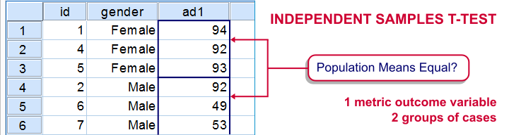
An independent samples t-test evaluates if 2 populations have equal means on some variable.
If the population means are really equal, then the sample means will probably differ a little bit but not too much. Very different sample means are highly unlikely if the population means are equal. This sample outcome thus suggest that the population means weren't equal after all.
The samples are independent because they don't overlap; none of the observations belongs to both samples simultaneously. A textbook example is male versus female respondents.
Example
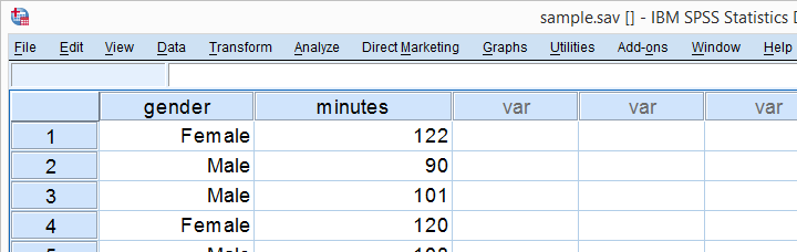
Some island has 1,000 male and 1,000 female inhabitants. An investigator wants to know if males spend more or fewer minutes on the phone each month. Ideally, he'd ask all 2,000 inhabitants but this takes too much time. So he samples 10 males and 10 females and asks them. Part of the data are shown below.
Next, he computes the means and standard deviations of monthly phone minutes for male and female respondents separately. The results are shown below.
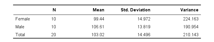
These sample means differ by some (99 - 106 =) -7 minutes: on average, females spend some 7 minutes less on the phone than males. But that's just our tiny samples. What can we say about the entire populations? We'll find out by starting off with the null hypothesis.
Null Hypothesis
The null hypothesis for an independent samples t-test is (usually) that the 2 population means are equal. If this is really true, then we may easily find slightly different means in our samples. So precisely what difference can we expect? An intuitive way for finding out is a simple simulation.
Simulation
I created a fake dataset containing the entire populations of 1,000 males and 1,000 females. On average, both groups spend 103 minutes on the phone with a standard-deviation of 14.5. Note that the null hypothesis of equal means is clearly true for these populations.
I then sampled 10 males and 10 females and computed the mean difference. And then I repeated that process 999 times, resulting in the 1,000 sample mean differences shown below.
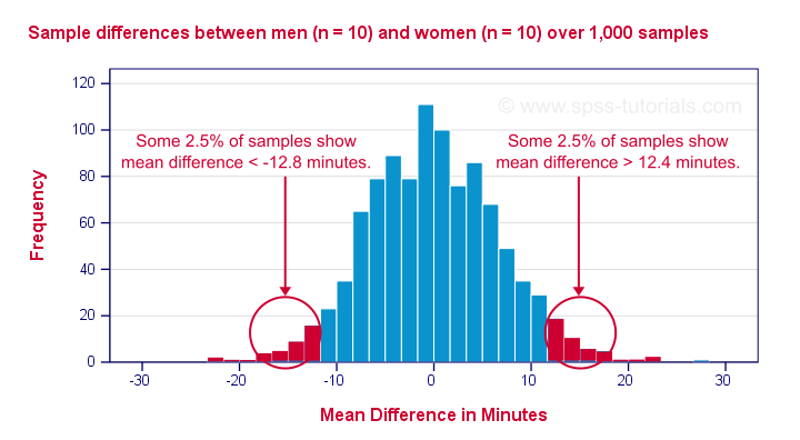
First off, the mean differences are roughly normally distributed. Most of the differences are close to zero -not surprising because the population difference is zero. But what's really interesting is that mean differences between, say, -12.5 and 12.5 are pretty common and make up 95% of my 1,000 outcomes. This suggests that an absolute difference of 12.5 minutes is needed for statistical significance at α = 0.05.
Last, the standard deviation of our 1,000 mean differences -the standard error- is 6.4. Note that some 95% of all outcomes lie between -2 and +2 standard errors of our (zero) mean. This is one of the best known rules of thumb regarding the normal distribution.
Now, an easier -though less visual- way to draw these conclusions is using a couple of simple formulas.
Test Statistic
Again: what is a “normal” sample mean difference if the population difference is zero? First off, this depends on the population standard deviation of our outcome variable. We don't usually know it but we can estimate it with
$$Sw = \sqrt{\frac{(n_1 - 1)\;S^2_1 + (n_2 - 1)\;S^2_2}{n_1 + n_2 - 2}}$$
in which \(Sw\) denotes our estimated population standard deviation.
For our data, this boils down to
$$Sw = \sqrt{\frac{(10 - 1)\;224 + (10 - 1)\;191}{10 + 10 - 2}} ≈ 14.4$$
Second, our mean difference should fluctuate less -that is, have a smaller standard error- insofar as our sample sizes are larger. The standard error is calculated as
$$Se = Sw\sqrt{\frac{1}{n_1} + \frac{1}{n_2}}$$
and this gives us
$$Se = 14.4\; \sqrt{\frac{1}{10} + \frac{1}{10}} ≈ 6.4$$
If the population mean difference is zero, then -on average- the sample mean difference will be zero as well. However, it will have a standard deviation of 6.4. We can now just compute a z-score for the sample mean difference but -for some reason- it's called T instead of Z:
$$T = \frac{\overline{X}_1 - \overline{X}_2}{Se}$$
which, for our data, results in
$$T = \frac{99.4 - 106.6}{6.4} ≈ -1.11$$
Right, now this is our test statistic: a number that summarizes our sample outcome with regard to the null hypothesis. T is basically the standardized sample mean difference; T = -1.11 means that our difference of -7 minutes is roughly 1 standard deviation below the average of zero.
Assumptions
Our t-value follows a t distribution but only if the following assumptions are met:
- Independent observations or, precisely, independent and identically distributed variables.
- Normality: the outcome variable follows a normal distribution in the population. This assumption is not needed for reasonable sample sizes (say, N > 25).
- Homogeneity: the outcome variable has equal standard deviations in our 2 (sub)populations. This is not needed if the sample sizes are roughly equal. Levene's test is sometimes used for testing this assumption.
If our data meet these assumptions, then T follows a t-distribution with (n1 + n2 -2) degrees of freedom (df). In our example, df = (10 + 10 - 2) = 18. The figure below shows the exact distribution. Note that we need an absolute t-value of 2.1 for 2-tailed significance at α = 0.05.
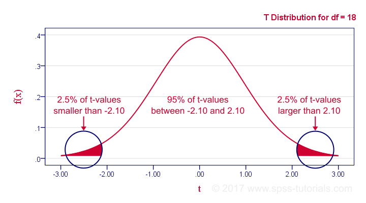
Minor note: as df becomes larger, the t-distribution approximates a standard normal distribution. The difference is hardly noticeable if df > 15 or so.
Statistical Significance
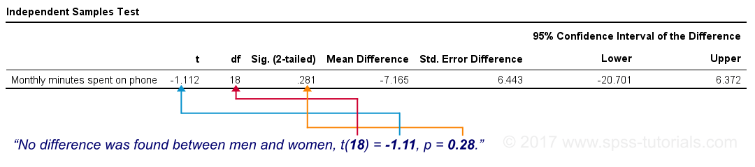
Last but not least, our mean difference of -7 minutes is not statistically significant: t(18) = -1.11, p ≈ 0.28. This means we've a 28% chance of finding our sample mean difference -or a more extreme one- if our population means are really equal; it's a normal outcome that doesn't contradict our null hypothesis.
Our final figure shows these results as obtained from SPSS.
Effect Size
Finally, the effect size measure that's usually preferred is Cohen’s D, defined as
$$D = \frac{\overline{X}_1 - \overline{X}_2}{Sw}$$
in which \(Sw\) is the estimated population standard deviation we encountered earlier. That is,
Cohen’s D is the number of standard deviations between the 2 sample means.
So what is a small or large effect? The following rules of thumb have been proposed:
- D = 0.20 indicates a small effect;
- D = 0.50 indicates a medium effect;
- D = 0.80 indicates a large effect.
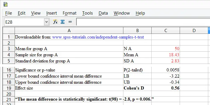
Cohen’s D is painfully absent from SPSS except for SPSS 27. However, you can easily obtain it from Cohens-d.xlsx. Just fill in 2 sample sizes, means and standard deviations and its formulas will compute everything you need to know.
Thanks for reading!
THIS TUTORIAL HAS 29 COMMENTS:
By dovys Arana on November 18th, 2018
Very helpful for all students.
By Alexandra Sigala on November 19th, 2018
THANK you for writing these guides. Saved my life (and my thesis!) Take care! <3
By William Peck on November 19th, 2018
In the spreadsheet, I plugged in my numbers in the top half, and the bottom half was all calculated. But the conclusion (“The mean difference is statistically significant: t(98) = -2.8, p = 0.006.”) looks hard-coded, is that right? Plus, how do you take the conclusion and present it to a manager?
By Ruben Geert van den Berg on November 20th, 2018
That's right. Rows 11-19 contain all formulas and will come up with all statistics such as statistical significance or p, effect size and so on.
Row 21 is merely a static example for how to report the results according to scientific guidelines. Perhaps I should make that clearer in the sheet itself. Last, "managers" don't always appreciate scientific guidelines. They often like to keep things simpler and rarely seem to care about more than just "significant" or "not significant". CTABLES offers some table options that are popular in corporate -rather than academic- environments.
Hope that helps!
By Illo A.I. on November 22nd, 2018
Thanks for the guides. It was really useful and helpful. How I wish you could something similar on Propensity score matching.
Kindly assist.
Regards