A probability density function is a function from which
probabilities for ranges of outcomes can be obtained.

• Probability Density Functions - Basic Rules
• Cumulative Probability Density Functions
• Inverse Cumulative Probability Density Functions
• Differences Probability Density and Probability Distributions
• Probability Density Functions in Applied Statistics

Example

The birth weights of mice follow a normal distribution, which is a probability density function. The population mean μ = 1 gram and the standard deviation σ = 0.25 grams. What's the probability that a newly born mouse
has a birth weight between 1.0 and 1.2 grams? The figure below shows how to obtain an approximate answer, using only the probability density curve we just described.

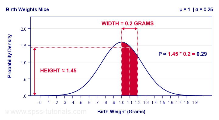
The probability is the surface area under the curve between 1.0 and 1.2 grams. It has a width of 0.2 grams and its average height -the probability density for this weight interval- is roughly 1.45. Therefore, the probability that a newborn mouse weighs between 1.0 and 1.2 grams is 1.45 · 0.2 = 0.29 -some 29%.

So What is Probability Density?

Probability density is probability per measurement unit. Our probability density of 1.45 means that the probability is 1.45 per gram -the measurement unit- over the interval between 1.0 and 1.2 grams. In contrast to probability, probability density can exceed 1 but only over an interval smaller than 1 measurement unit.

Compare this to population density: a population density of 100 inhabitants per square kilometer for some village doesn't imply that it has 100 inhabitants. If this village has a surface area of only 0.5 square kilometers, then it has (100 · 0.5 =) 50 inhabitants.

The screenshot below shows how to get a probability density from Excel or Google sheets.

Simply typing =NORM.DIST(1.1,1,0.25,FALSE) into some cell returns the probability density at x = 1.1, which is 1.473. The last argument, cumulative, refers to the cumulative density function which we'll discuss in a minute.

Anyway. In applied statistics, we're usually after probabilities instead of probability densities. So what good is a curve showing probability densities? Well, just like a histogram, it shows which ranges of values occur how often. Like so, it predicts what a histogram will look like if we actually draw a (reasonably large) sample.
The figure below illustrates just this: it shows a histogram for a sample of 10,000 mice with the assumed normal curve (in red) superimposed on it.

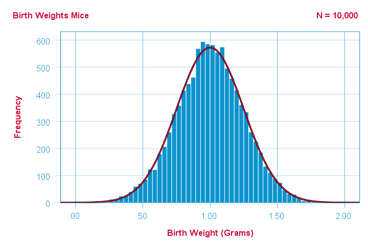The normal curve (in red) predicts the shape of this histogram fairly precisely.

This curve -just a simple function- gives us a ton of information about our variable such as its

• mean;
• median;
• standard deviation, skewness, kurtosis, interquartile range and more.

Probability Density Functions - Basic Rules

The mathematical definition of a probability density function is any function

• whose surface area is 1 and
• which doesn't return values < 0.

Furthermore,

• probability density functions only apply to continuous variables and
• the probability for any single outcome is defined as zero. Only ranges of outcomes have non zero probabilities.

So how do we usually obtain such probabilities in applied research? The easy way is using a cumulative probability density function.

Cumulative Probability Density Functions

A cumulative probability density function returns the probability
that an outcome is smaller than some value x. Such a probability -denoted as \(P(X \lt x)\)- is known as a cumulative probability.

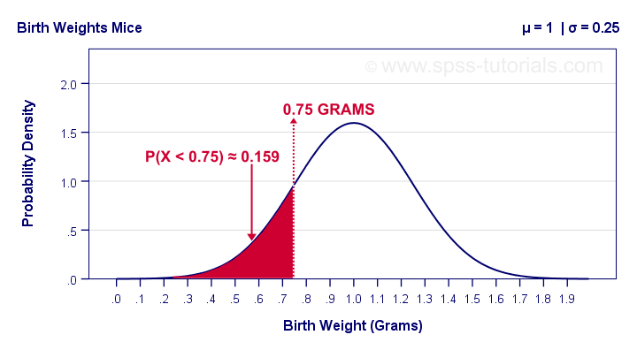
Example: the birth weights of mice are normally distributed with μ = 1 and σ = 0.25 grams. What's the probability that a random mouse is born with a weight less than 0.75 grams? The figure below shows that this probability corresponds to the surface area left of 0.75 grams, which is 0.159 or 15.9%.

So how did we find this exact surface area? Well, the surface area left of any value can be computed with an integral:

$$F_{cpd}(x) = \int_{-\infty}^x F_{pd}(x)dx = P(X \lt x)$$

where

• \(F_{cpd}(x)\) denotes the cumulative probability density function;
• \(F_{pd}(x)\) denotes a probability density function and
• \(P(X \lt x)\) is the probability that an outcome \(X \lt x\).

The figure below shows what a cumulative normal density function looks like.

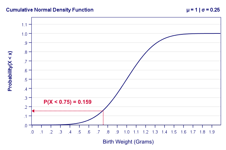
Note that we can readily look up probabilities from this curve. However, we can't easily estimate this variable's mean, standard deviation or skewness from this curve. The main exception to this is its median of 1.0 grams.
Last but not least, the screenshot below shows how to obtain cumulative probabilities in Excel or Google Sheets.

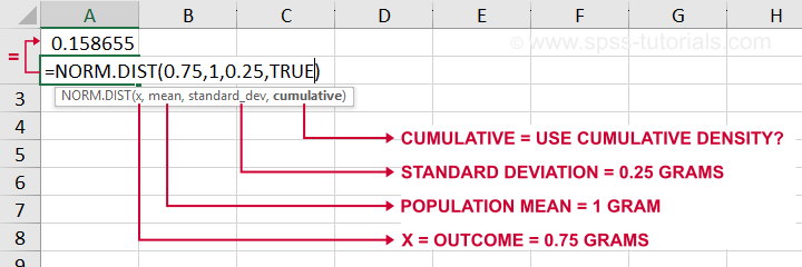
If a variable is normally distributed with μ = 1 and σ = 0.25, then typing =NORM.DIST(0.75,1,0.25,TRUE) into some cell returns the probability that X < 0.75, which is 0.159.

Inverse Cumulative Probability Density Functions

An inverse cumulative probability density function returns
the value x for a given cumulative probability. Example: the birth weights of mice are normally distributed with μ = 1 and σ = 0.25 grams. Which birth weight separates the 10% lowest from the 90% highest birth weights? The figure below shows how to find this value in Excel: a birth weight less than 0.680 grams has a 0.1 or 10% probability of occurring.

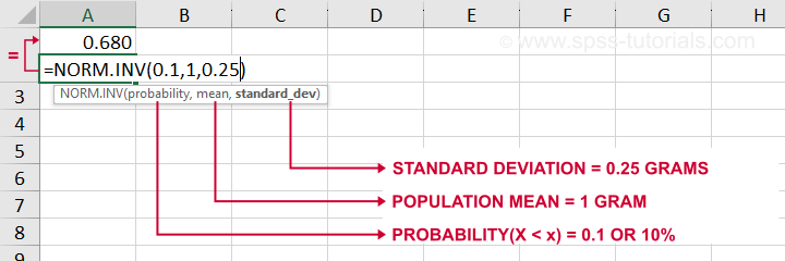
Looking up this value from the inverse cumulative density in Excel is done by typing =NORM.INV(0.1,1,0.25) which returns a value (birth weight in this example) of 0.680.

Differences Probability Density and Probability Distributions

Probability density functions are often misreferred to as “probability-distributions”. This is confusing because they really are 2 different things:

• probability density functions apply to continuous variables whereas probability distributions apply to discrete variables;
• probability density functions return probability densities whereas probability distribution functions return probabilities;
• by definition, separate outcomes have zero probabilities for probability density functions. For probability distributions, separate outcomes may have non zero probabilities.

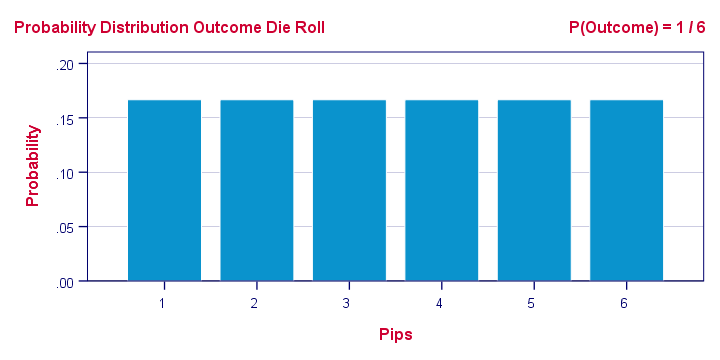
A text book illustration of a true probability distribution is shown below: the outcome of a roll with a balanced die.

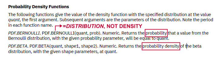
Sadly, the SPSS manual abbreviates both density and distribution functions to “PDF” as shown below. Also note that the Bernoulli distribution -a probability distribution- is wrongfully listed under probability density functions.

Interestingly, cumulative probability density functions are comparable to cumulative probability functions. Both return cumulative probabilities: the probability that some outcome is equal to or smaller than some value x denoted as \(P(X \le x)\).

Probability Density Functions in Applied Statistics

The big 4 probability density functions in applied statistics are

• the normal distribution (normality assumption and z-tests);
• the t-distribution (t-tests and regression coefficients);
• the χ²-distribution (chi-square test and loglinear analysis);
• the F-distribution (ANOVA, Levene's test).

These functions are used in different forms that serve different purposes:

1. Cumulative probability density functions return probabilities for ranges of outcomes. Two such types of probabilities are

• statistical significance and
• (1 - β) or power.

2. Inverse cumulative probability density functions return ranges of outcomes for (chosen) probabilities. Like so, they're used for constructing confidence intervals: ranges of values that enclose some parameter with a given likelihood, often 95%. Example: “the 95% confidence interval for the mean monthly salary runs from $2,300 through $2,450”.

3. Probability density functions are sometimes used to inspect statistical assumptions. Like so, the normality assumption can be evaluated by superimposing a normal curve over a histogram of observed values like we saw here. Alternatives for testing for normality are

• the Shapiro-Wilk test and
• the Kolmogorov-Smirnov test.

Right. I guess that's basically it regarding probability density functions. Let us know if you found this tutorial helpful by throwing a comment below.

Thanks for reading!