An assumption required for ANOVA is homogeneity of variances. We often run Levene’s test to check if this holds. But what if it doesn't? This tutorial walks you through.
- SPSS ANOVA Dialogs I
- Results I - Levene’s Test “Significant“
- SPSS ANOVA Dialogs II
- Results II - Welch and Games-Howell Tests
- Plan B - Kruskal-Wallis Test
Example Data
All analyses in this tutorial use staff.sav, part of which is shown below. We encourage you to download these data and replicate our analyses.
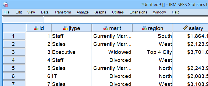
Our data contain some details on a sample of N = 179 employees. The research question for today is: is salary associated with region? We'll try to support this claim by rejecting the null hypothesis that all regions have equal mean population salaries. A likely analysis for this is an ANOVA but this requires a couple of assumptions.
ANOVA Assumptions
An ANOVA requires 3 assumptions:
- independent observations;
- normality: the dependent variable must follow a normal distribution within each subpopulation.
- homogeneity: the variance of the dependent variable must be equal over all subpopulations.
With regard to our data, independent observations seem plausible: each record represents a distinct person and people didn't interact in any way that's likely to affect their answers.
Second, normality is only needed for small sample sizes of, say, N < 25 per subgroup. We'll inspect if our data meet this requirement in a minute.
Last, homogeneity is only needed if sample sizes are sharply unequal. If so, we usually run Levene's test. This procedure tests if 2+ population variances are all likely to be equal.
Quick Data Check
Before running our ANOVA, let's first see if the reported salaries are even plausible. The best way to do so is inspecting a histogram which we'll create by running the syntax below.
frequencies salary
/format notable
/histogram.
Result
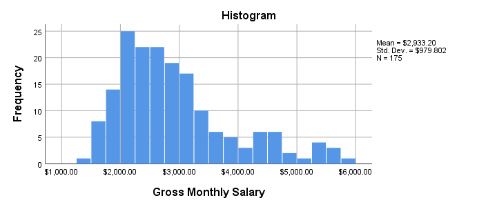
- Note that our histogram reports N = 175 rather than our N = 179 respondents. This implies that salary contains 4 missing values.
- The frequency distribution, however, looks plausible: there's no clear outliers or other abnormalities that should ring any alarm bells.
- The distribution shows some positive skewness. However, this makes perfect sense and is no cause for concern.
Let's now proceed to the actual ANOVA.
SPSS ANOVA Dialogs I
After opening our data in SPSS, let's first navigate to
![]()
![]() as shown below.
as shown below.
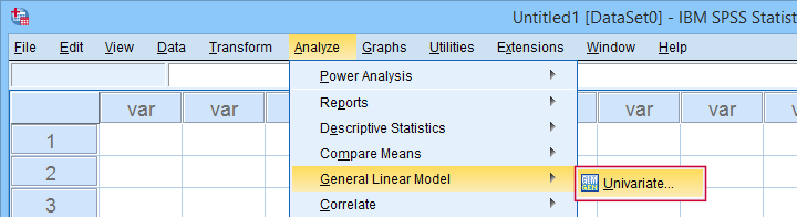
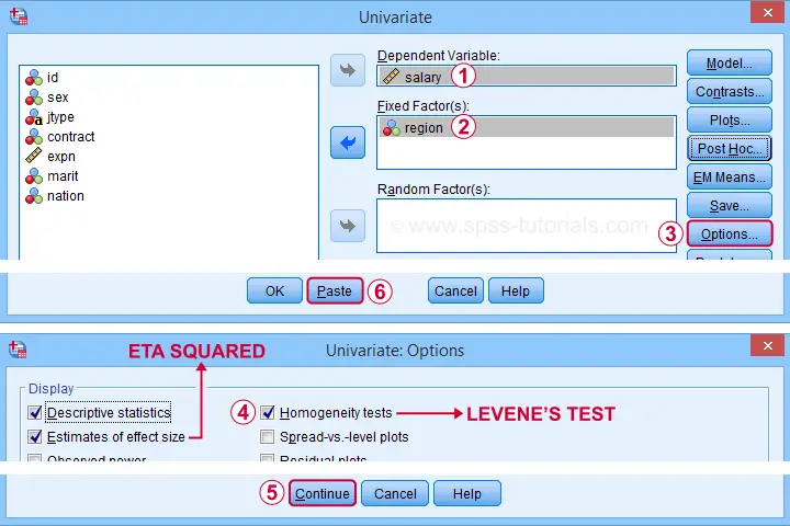
Let's now fill in the dialog that opens as shown below.
Completing these steps results in the syntax below. Let's run it.
UNIANOVA salary BY region
/METHOD=SSTYPE(3)
/INTERCEPT=INCLUDE
/PRINT ETASQ DESCRIPTIVE HOMOGENEITY
/CRITERIA=ALPHA(.05)
/DESIGN=region.
Results I - Levene’s Test “Significant”
The very first thing we inspect are the sample sizes used for our ANOVA and Levene’s test as shown below.
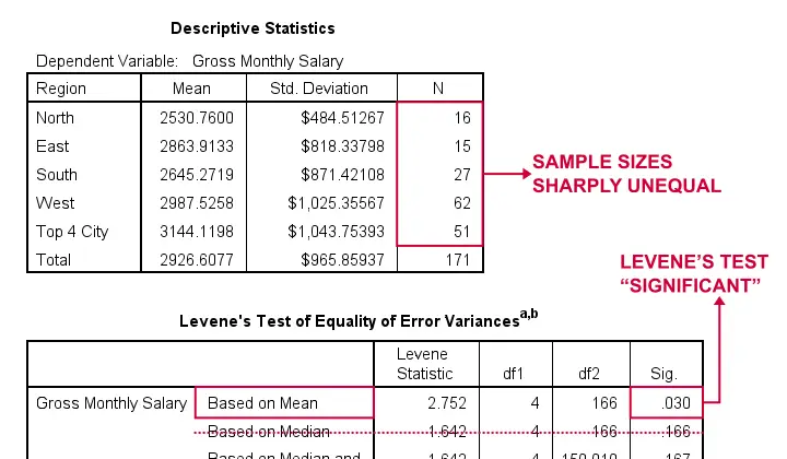
- First off, note that our Descriptive Statistics table is based on N = 171 respondents (bottom row). This is due to some missing values in both region and salary.
- Second, sample sizes for “North” and “East” are rather small. We may therefore need the normality assumption. For now, let's just assume it's met.
- Next, our sample sizes are sharply unequal so we really need to meet the homogeneity of variances assumption.
- However, Levene’s test is statistically significant because its p < 0.05: we reject its null hypothesis of equal population variances.
The combination of these last 2 points implies that we can not interpret or report the F-test shown in the table below.
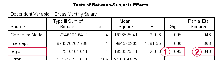
 As discussed, we can't rely on this p-value for the usual F-test.
 However, we can still interpret eta squared (often written as η2). This is a descriptive statistic that neither requires normality nor homogeneity. η2 = 0.046 implies a small to medium effect size for our ANOVA.
Now, if we can't interpret our F-test, then how can we know if our mean salaries differ? Two good alternatives are:
- running an ANOVA with the Welch statistic or
- a Kruskal-Wallis test.
Let's start off with the Welch statistic.
SPSS ANOVA Dialogs II
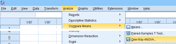
For inspecting the Welch statistic, first navigate to
![]()
![]() as shown below.
as shown below.
Next, we'll fill out the dialogs that open as shown below.
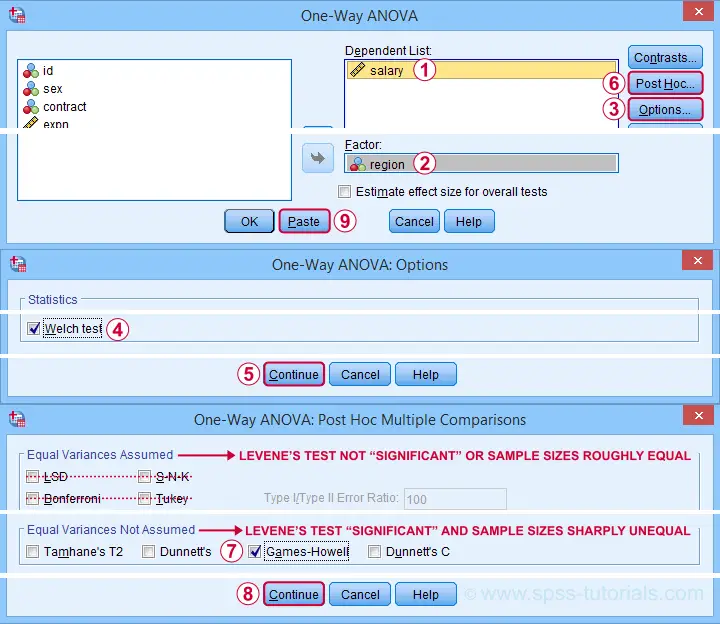
This results in the syntax below. Again, let's run it.
ONEWAY salary BY region
/STATISTICS HOMOGENEITY WELCH
/MISSING ANALYSIS
/POSTHOC=GH ALPHA(0.05).
Results II - Welch and Games-Howell Tests
As shown below, the Welch test rejects the null hypothesis of equal population means.
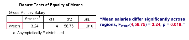
This table is labelled “Robust Tests...” because it's robust to a violation of the homogeneity assumption as indicated by Levene’s test. So we now conclude that mean salaries are not equal over all regions.
But precisely which regions differ with regard to mean salaries? This is answered by inspecting post hoc tests. And if the homogeneity assumption is violated, we usually prefer Games-Howell as shown below.
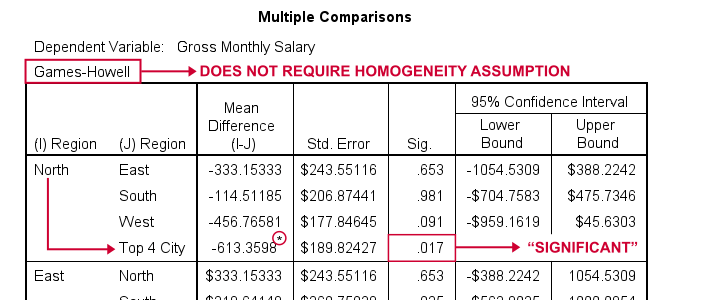
Note that each comparison is shown twice in this table. The only regions whose mean salaries differ “significantly” are North and Top 4 City.
Plan B - Kruskal-Wallis Test
So far, we overlooked one issue: some regions have sample sizes of n = 15 or n = 16. This implies that the normality assumption should be met as well. A terrible idea here is to run
for each region separately. Neither test rejects the null hypothesis of a normally distributed dependent variable but this is merely due to insufficient sample sizes.
A much better idea is running a Kruskal-Wallis test. You could do so with the syntax below.
NPAR TESTS
/K-W=salary BY region(1 5)
/STATISTICS DESCRIPTIVES
/MISSING ANALYSIS.
Result
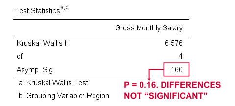
Sadly, our Kruskal-Wallis test doesn't detect any difference between mean salary ranks over regions, H(4) = 6.58, p = 0.16.
In short, our analyses come up with inconclusive outcomes and it's unclear precisely why. If you've any suggestions, please throw us a comment below. Other than that,
Thanks for reading!
THIS TUTORIAL HAS 13 COMMENTS:
By Ruben Geert van den Berg on August 12th, 2022
Hi YY, thanks for your suggestions!
However, I'm not too concerned about normality -especially for the last 3 groups. My guess is that the central limit theory takes care of that.
I really have a problem with normalizing transformations: different analysts may choose different transformations with different parameters (which power? which constant?) and these affect the shapes of the resulting distributions and -hence- the final conclusions.
This induces a degree of subjectivity into the results: try different transformations until you find what you want to find.
On the other hand, if all options converge regarding results, that does constitute stronger evidence than a single procedure.
For the data at hand, I guess the results remain somewhat inconclusive at best -also an outcome...
By Jon Peck on August 13th, 2023
The Welch test has very good power - close to the t/F test even with equal variances, so there is very little lost by skipping the variance test and just using Welch all the time compared to a test and choose strategy. (Or Brown-forsythe).
By Ndamsa nelson on March 20th, 2025
how do i code my questionnaire into spss for ANOVA Analysis