• Descriptive Statistics for Subgroups
• ANOVA - Flowchart
• SPSS ANOVA Dialogs
• SPSS ANOVA Output
• SPSS ANOVA - Post Hoc Tests Output
• APA Style Reporting Post Hoc Tests

Post hoc tests in ANOVA test if the difference between
each possible pair of means is statistically significant. This tutorial walks you through running and understanding post hoc tests using depression.sav, partly shown below.

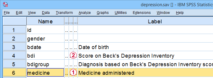
The variables we'll use are

the medicine that our participants were randomly assigned to and
their levels of depressiveness measured 16 weeks after starting medication.

Our research question is whether some medicines result in lower depression scores than others. A better analysis here would have been ANCOVA but -sadly- no depression pretest was administered.

Quick Data Check

Before jumping blindly into any analyses, let's first see if our data look plausible in the first place. A good first step is inspecting a histogram which I'll run from the SPSS syntax below.

Result

First off, our histogram (shown below) doesn't show anything surprising or alarming.

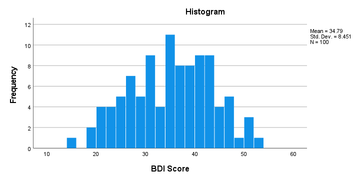
Also, note that N = 100 so this variable does not have any missing values. Finally, it could be argued that a single participant near 15 points could be an outlier. It doesn't look too bad so we'll just leave it for now.

Descriptive Statistics for Subgroups

Let's now run some descriptive statistics for each medicine group separately. The right way for doing so is from Analyze Compare Means Means or simply typing the 2 lines of syntax shown below.

Result

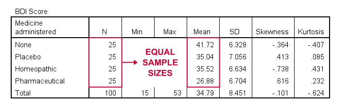
As shown, I like to present a nicely detailed table including the

• mean,
• median (omitted here),
• standard deviation,
• skewness and
• kurtosis

for each group separately. But most important here are the sample sizes because these affect which assumptions we'll need for our ANOVA.

Also note that the mean depression scores are quite different across medicines. However, these are based on rather small samples. So the big question is: what can we conclude about the entire populations? That is: all people who'll take these medicines?

ANOVA - Null Hypothesis

In short, our ANOVA tries to demonstrate that some medicines work better than others by nullifying the opposite claim. This null hypothesis states that the population mean depression scores are equal
across all medicines. An ANOVA will tell us if this is credible, given the sample data we're analyzing. However, these data must meet a couple of assumptions in order to trust the ANOVA results.

ANOVA - Assumptions

ANOVA requires the following assumptions:

• independent observations;
• normality: the dependent variable must be normally distributed within each subpopulation we're comparing. However, normality is not needed if each n > 25 or so.
• homogeneity: the variance of the dependent variable must be equal across all subpopulations we're comparing. However, homogeneity is not needed if all sample sizes are roughly equal.

Now, homogeneity is only required for sharply unequal sample sizes. In this case, Levene's test can be used to examine if homogeneity is met. What to do if it isn't, is covered in SPSS ANOVA - Levene’s Test “Significant”.

ANOVA - Flowchart

The flowchart below summarizes when/how to check the ANOVA assumptions and what to do if they're violated.

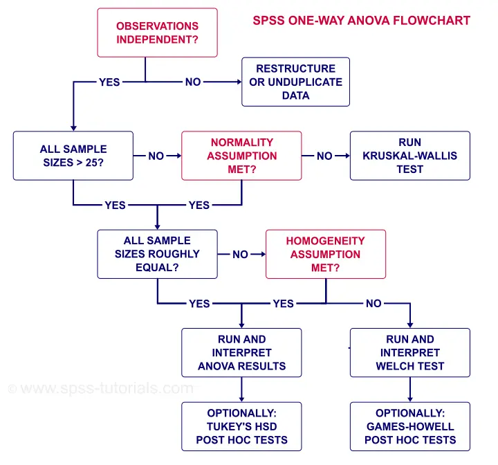
Note that depression.sav contains 4 medicine samples of n = 25 independent observations. It therefore meets all ANOVA assumptions.

SPSS ANOVA Dialogs

We'll run our ANOVA from Analyze Compare Means One-Way ANOVA as shown below.

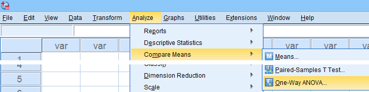
Next, let's fill out the dialogs as shown below.

Estimate effect size(...) is only available for SPSS version 27 or higher. If you're on an older version, you can get it from Analyze Compare Means Means (“ANOVA table” under “Options”).

Tukey's HSD (“honestly significant difference”) is the most common post hoc test for ANOVA. It is listed under “equal variances assumed”, which refers to the homogeneity assumption. However, this is not needed for our data because our sample sizes are all equal.

Completing these steps results in the syntax below.

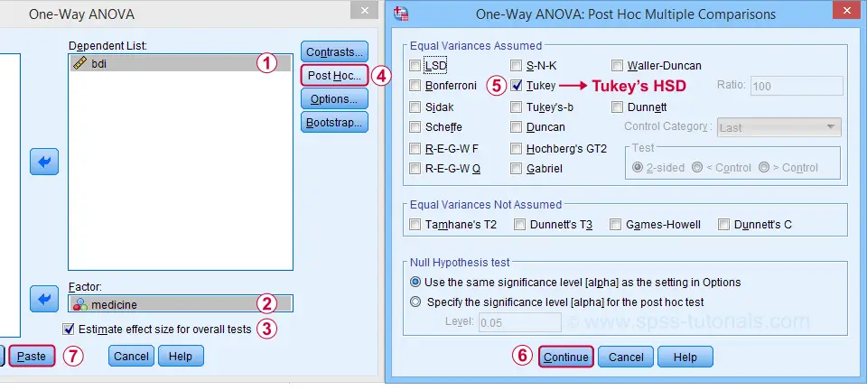
SPSS ANOVA Output

First off, the ANOVA table shown below addresses the null hypothesis that all population means are equal. The significance level indicates that p < .001 so we reject this null hypothesis. The figure below illustrates how this result should be reported.

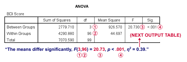
What's absent from this table, is eta squared, denoted as η². In SPSS 27 and higher, we find this in the next output table shown below.

Eta-squared is an effect size measure: it is a single, standardized number that expresses how different several sample means are (that is, how far they lie apart). Generally accepted rules of thumb for eta-squared are that

• η² = 0.01 indicates a small effect;
• η² = 0.06 indicates a medium effect;
• η² = 0.14 indicates a large effect.

For our example, η² = 0.39 is a huge effect: our 4 medicines resulted in dramatically different mean depression scores.

This may seem to complete our analysis but there's one thing we don't know yet: precisely which mean differs from which mean? This final question is answered by our post hoc tests that we'll discuss next.

SPSS ANOVA - Post Hoc Tests Output

The table below shows if the difference between each pair of means is statistically significant. It also includes 95% confidence intervals for these differences.

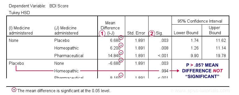
Mean differences that are “significant” at our chosen α = .05 are flagged. Note that each mean differs from each other mean except for Placebo versus Homeopathic.

If we take a good look at the exact 2-tailed p-values, we see that they're all < .01 except for the aforementioned comparison.

Given this last finding, I suggest rerunning our post hoc tests at α = .01 for reconfirming these findings. The syntax below does just that.

APA Style Reporting Post Hoc Tests

The table below shows how to report post hoc tests in APA style.

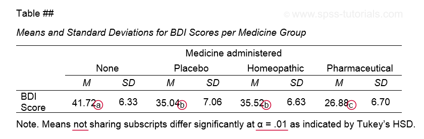
This table itself was created with a MEANS command like we used for Descriptive Statistics for Subgroups. The subscripts are based on the Homogeneous Subsets table in our ANOVA output.

Note that we chose α = .01 instead of the usual α = .05. This is simply more informative for our example analysis because all of our p-values < .05 are also < .01.

This APA table also seems available from Analyze Tables Custom Tables but I don't recommend this: the p-values from Custom Tables seem to be based on Bonferroni adjusted independent samples t-tests instead of Tukey's HSD. The general opinion on this is that this procedure is overly conservative.

Final Notes

Right, so a common routine for ANOVA with post hoc tests is

1. run a basic ANOVA to see if the population means are all equal. This is often referred to as the omnibus test (omnibus is Latin, meaning something like “about all things”);
2. only if we reject this overall null hypothesis, then find out precisely which pairs of means differ with post hoc tests (post hoc is Latin for “after that”).

Running post hoc tests when the omnibus test is not statistically significant is generally frowned upon. Some scenarios could perhaps justify doing so but let's leave that discussion for another day.

Right, so that should do. I hope you found this tutorial helpful. If you've any questions or remarks, please throw me a comment below. Other than that...

thanks for reading!