SPSS Missing Values Tutorial

Contents

• SPSS System Missing Values
• SPSS User Missing Values
• Setting User Missing Values
• Inspecting Missing Values per Variable
• SPSS Data Analysis with Missing Values

What are “Missing Values” in SPSS?

In SPSS, “missing values” may refer to 2 things:

• System missing values are values that are completely absent from the data. They are shown as periods in data view.
• User missing values are values that are invisible while analyzing or editing data. The SPSS user specifies which values -if any- must be excluded.

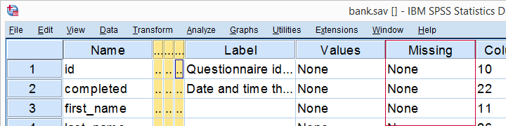
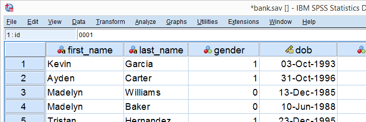
This tutorial walks you through both. We'll use bank.sav -partly shown below- throughout. You'll get the most out of this tutorial if you try the examples for yourself after downloading and opening this file.

SPSS System Missing Values

System missing values are values that are
completely absent from the data. System missing values are shown as dots in data view as shown below.

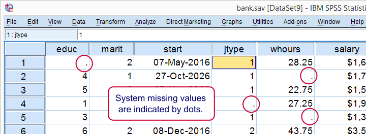
System missing values are only found in numeric variables. String variables don't have system missing values. Data may contain system missing values for several reasons:

• some respondents weren't asked some questions due to the questionnaire routing;
• a respondent skipped some questions;
• something went wrong while converting or editing the data;
• some values weren't recorded due to equipment failure.

In some cases system missing values make perfect sense. For example, say I ask “do you own a car?” and somebody answers “no”. Well, then my survey software should skip the next question: “what color is your car?” In the data, we'll probably see system missing values on color for everyone who does not own a car. These missing values make perfect sense.
In other cases, however, it may not be clear why there's system missings in your data. Something may or may not have gone wrong. Therefore, you should try to find out why some values are system missing especially if there's many of them.
So how to detect and handle missing values in your data? We'll get to that after taking a look at the second type of missing values.

SPSS User Missing Values

User missing values are values that are excluded
when analyzing or editing data. “User” in user missing refers to the SPSS user. Hey, that's you! So it's you who may need to set some values as user missing. So which -if any- values must be excluded? Briefly,

• for categorical variables, answers such as “don't know” or “no answer” are typically excluded from analysis.
• For metric variables, unlikely values -a reaction time of 50ms or a monthly salary of € 9,999,999- are usually set as user missing.

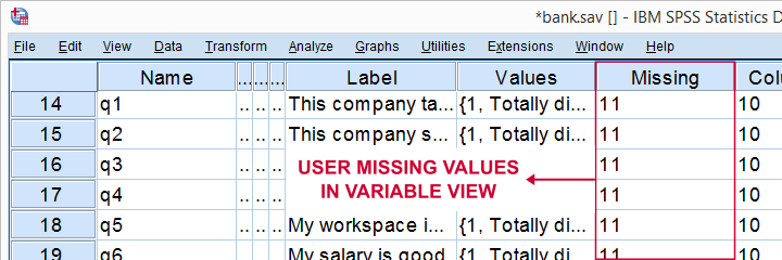
For bank.sav, no user missing values have been set yet, as can be seen in variable view.

Let's now see if any values should be set as user missing and how to do so.

User Missing Values for Categorical Variables

A quick way for inspecting categorical variables is running frequency distributions and corresponding bar charts. Make sure the output tables show both values and value labels. The easiest way for doing so is running the syntax below.

Result

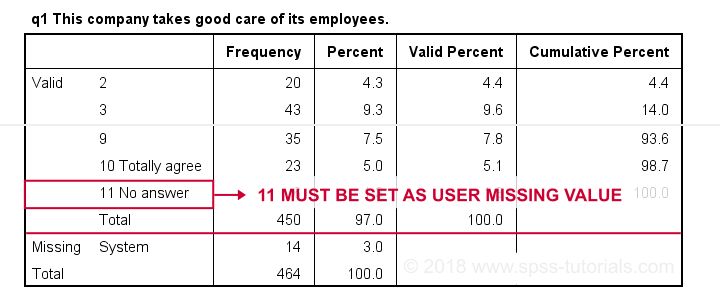
First note that q1 is an ordinal variable: higher values indicate higher levels of agreement. However, this does not go for 11: “No answer” does not indicate more agreement than 10 - “Totally agree”. Therefore, only values 1 through 10 make up an ordinal variable and 11 should be excluded.
The syntax below shows the right way to do so.

Result

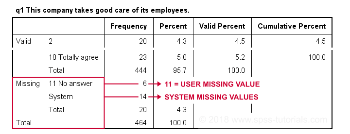
Note that 11 is shown among the missing values now. It occurs 6 times in q1 and there's also 14 system missing values. In variable view, we also see that 11 is set as a user missing value for q1 through q9.

User Missing values for Metric Variables

The right way to inspect metric variables is running histograms over them. The syntax below shows the easiest way to do so.

Result

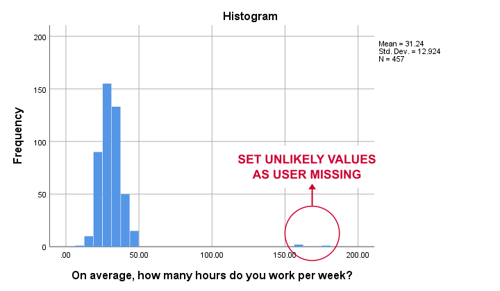
Some respondents report working over 150 hours per week. Perhaps these are their monthly -rather than weekly- hours. In any case, such values are not credible. We'll therefore set all values of 50 hours per week or more as user missing. After doing so, the distribution of the remaining values looks plausible.

Inspecting Missing Values per Variable

A super fast way to inspect (system and user) missing values per variable is running a basic DESCRIPTIVES table. Before doing so, make sure you don't have any WEIGHT or FILTER switched on. You can check this by running SHOW WEIGHT FILTER N. Also note that there's 464 cases in these data. So let's now inspect the descriptive statistics.

Result

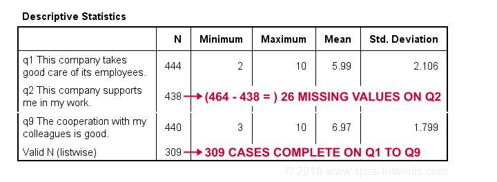
The N column shows the number of non missing values per variable. Since we've 464 cases in total, (464 - N) is the number of missing values per variable. If any variables have high percentages of missingness, you may want to exclude them from -especially- multivariate analyses.
Importantly, note that Valid N (listwise) = 309. These are the cases without any missing values on all variables in this table. Some procedures will use only those 309 cases -known as listwise exclusion of missing values in SPSS.
Conclusion: none of our variables -columns of cells in data view- have huge percentages of missingness. Let's now see if any cases -rows of cells in data view- have many missing values.

Inspecting Missing Values per Case

For inspecting if any cases have many missing values, we'll create a new variable. This variable holds the number of missing values over a set of variables that we'd like to analyze together. In the example below, that'll be q1 to q9.
We'll use a short and simple variable name: mis_1 is fine. Just make sure you add a description of what's in it -the number of missing...- as a variable label.

Result

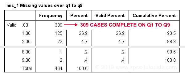
In this table, 0 means zero missing values over q1 to q9. This holds for 309 cases. This is the Valid N (listwise) we saw in the descriptives table earlier on.
Also note that 1 case has 8 missing values out of 9 variables. We may doubt if this respondent filled out the questionnaire seriously. Perhaps we'd better exclude it from the analyses over q1 to q9. The right way to do so is using a FILTER.

SPSS Data Analysis with Missing Values

So how does SPSS analyze data if they contain missing values? Well, in most situations, SPSS runs each analysis on all cases it can use for it. Right, now our data contain 464 cases. However, most analyses can't use all 464 because some may drop out due to missing values. Which cases drop out depends on which analysis we run on which variables.
Therefore, an important best practice is to always inspect how many cases are actually used
for each analysis you run. This is not always what you might expect. Let's first take a look at pairwise exclusion of missing values.

Pairwise Exclusion of Missing Values

Let's inspect all (Pearson) correlations among q1 to q9. The simplest way for doing so is just running correlations q1 to q9. If we do so, we get the table shown below.

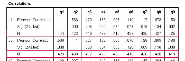
Note that each correlation is based on a different number of cases. Precisely, each correlation between a pair of variables uses all cases having valid values on these 2 variables. This is known as pairwise exclusion of missing values. Note that most correlations are based on some 410 up to 440 cases.

Listwise Exclusion of Missing Values

Let's now rerun the same correlations after adding a line to our minimal syntax: correlations q1 to q9
/missing listwise. After running it, we get a smaller correlation matrix as shown below. It no longer includes the number of cases per correlation.

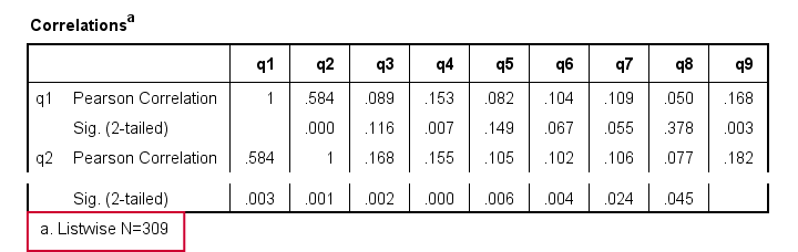
Each correlation is based on the same 309 cases, the listwise N. These are the cases without missing values on all variables in the table: q1 to q9. This is known as listwise exclusion of missing values.
Obviously, listwise exclusion often uses far fewer cases than pairwise exclusion. This is why we often recommend the latter: we want to use as many cases as possible. However, if many missing values are present, pairwise exclusion may cause computational issues. In any case, make sure you know if your analysis uses
listwise or pairwise exclusion of missing values. By default, regression and factor analysis use listwise exclusion and in most cases, that's not what you want.

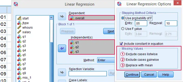
Exclude Missing Values Analysis by Analysis

Analyzing if 2 variables are associated is known as bivariate analysis. When doing so, SPSS can only use cases having valid values on both variables. Makes sense, right?
Now, if you run several bivariate analyses in one go, you can exclude cases analysis by analysis: each separate analysis uses all cases it can. Different analyses may use different subsets of cases.
If you don't want that, you can often choose listwise exclusion instead: each analysis uses only cases without missing values on all variables for all analyses. The figure below illustrates this for ANOVA.

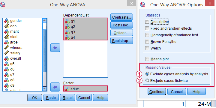
The test for q1 and educ uses all cases having valid values on q1 and educ, regardless of q2 to q4.
All tests use only cases without missing values on q1 to q4 and educ.

We usually want to use as many cases as possible for each analysis. So we prefer to exclude cases analysis by analysis. But whichever you choose, make sure you know how many cases are used for each analysis. So check your output carefully. The Kolmogorov-Smirnov test is especially tricky in this respect: by default, one option excludes cases analysis by analysis and the other uses listwise exclusion.

Editing Data with Missing Values

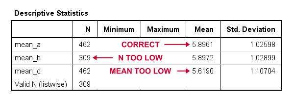
Editing data with missing values can be tricky. Different commands and functions act differently in this case. Even something as basic as computing means in SPSS can go very wrong if you're unaware of this.
The syntax below shows 3 ways we sometimes encounter. With missing values, however, 2 of those yield incorrect results.

Result

Final Notes

In real world data, missing values are common. They don't usually cause a lot of trouble when analyzing or editing data but in some cases they do. A little extra care often suffices if missingness is limited. Double check your results and know what you're doing.

Thanks for reading.

SPSS Factor Analysis – Beginners Tutorial

• What is Factor Analysis?
• Quick Data Checks
• Running Factor Analysis in SPSS
• SPSS Factor Analysis Output
• Adding Factor Scores to Our Data

What is Factor Analysis?

Factor analysis examines which underlying factors are measured
by a (large) number of observed variables. Such “underlying factors” are often variables that are difficult to measure such as IQ, depression or extraversion. For measuring these, we often try to write multiple questions that -at least partially- reflect such factors. The basic idea is illustrated below.

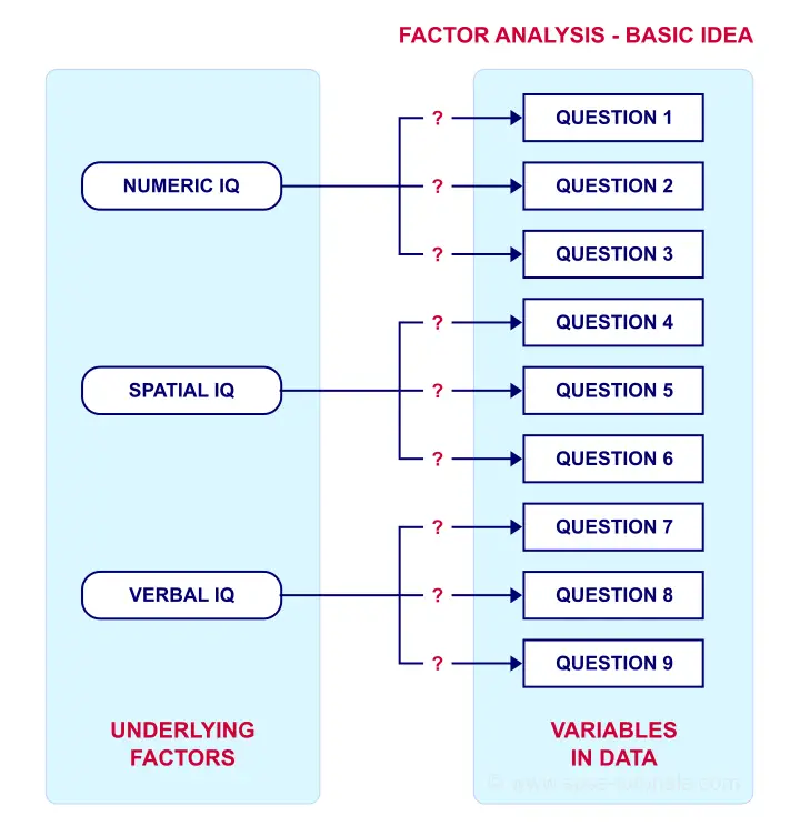
Now, if questions 1, 2 and 3 all measure numeric IQ, then the Pearson correlations among these items should be substantial: respondents with high numeric IQ will typically score high on all 3 questions and reversely.

The same reasoning goes for questions 4, 5 and 6: if they really measure “the same thing” they'll probably correlate highly.

However, questions 1 and 4 -measuring possibly unrelated traits- will not necessarily correlate. So if my factor model is correct, I could expect the correlations to follow a pattern as shown below.

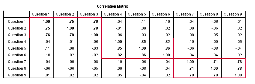
Confirmatory Factor Analysis

Right, so after measuring questions 1 through 9 on a simple random sample of respondents, I computed this correlation matrix. Now I could ask my software if these correlations are likely, given my theoretical factor model. In this case, I'm trying to confirm a model by fitting it to my data. This is known as “confirmatory factor analysis”.

SPSS does not include confirmatory factor analysis but those who are interested could take a look at AMOS.

Exploratory Factor Analysis

But what if I don't have a clue which -or even how many- factors are represented by my data? Well, in this case, I'll ask my software to suggest some model given my correlation matrix. That is, I'll explore the data (hence, “exploratory factor analysis”). The simplest possible explanation of how it works is that the software tries to find groups of variables
that are highly intercorrelated. Each such group probably represents an underlying common factor. There's different mathematical approaches to accomplishing this but the most common one is principal components analysis or PCA. We'll walk you through with an example.

Research Questions and Data

A survey was held among 388 applicants for unemployment benefits. The data thus collected are in dole-survey.sav, part of which is shown below.

The survey included 16 questions on client satisfaction. We think these measure a smaller number of underlying satisfaction factors but we've no clue about a model. So our research questions for this analysis are:

• how many factors are measured by our 16 questions?
• which questions measure similar factors?
• which satisfaction aspects are represented by which factors?

Quick Data Checks

Now let's first make sure we have an idea of what our data basically look like. We'll inspect the frequency distributions with corresponding bar charts for our 16 variables by running the syntax below.

Result

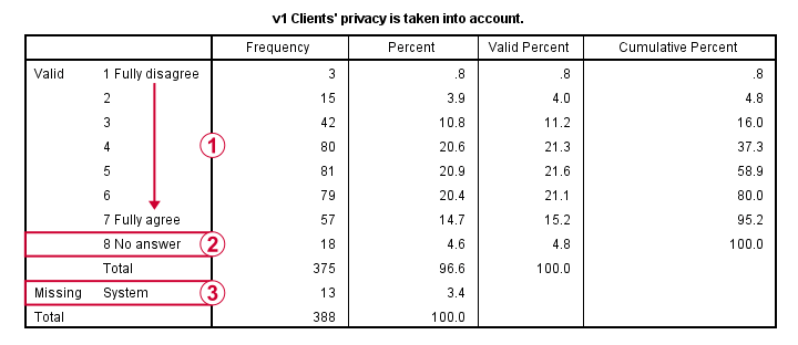
This very minimal data check gives us quite some important insights into our data:

• All frequency distributions look plausible. We don't see anything weird in our data.
• All variables are positively coded: higher values always indicate more positive sentiments.
• All variables have a value 8 (“No answer”) which we need to set as a user missing value.
• All variables have some system missing values too but the extent of missingness isn't too bad.

A somewhat annoying flaw here is that we don't see variable names for our bar charts in the output outline.

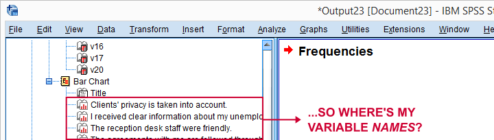
If we see something unusual in a chart, we don't easily see which variable to address. But in this example -fortunately- our charts all look fine.

So let's now set our missing values and run some quick descriptive statistics with the syntax below.

Result

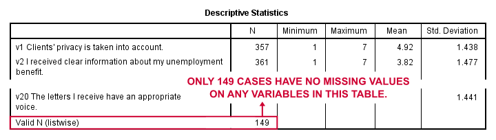
Note that none of our variables have many -more than some 10%- missing values. However, only 149 of our 388 respondents have zero missing values on the entire set of variables. This is very important to be aware of as we'll see in a minute.

Running Factor Analysis in SPSS

Let's now navigate to Analyze Dimension Reduction Factor as shown below.

In the dialog that opens, we have a ton of options. For a “standard analysis”, we'll select the ones shown below. If you don't want to go through all dialogs, you can also replicate our analysis from the syntax below.

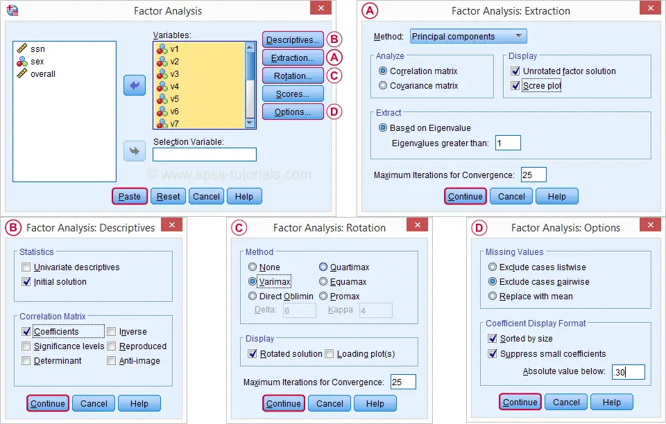
Avoid “Exclude cases listwise” here as it'll only include our 149 “complete” respondents in our factor analysis. Clicking Paste results in the syntax below.

SPSS Factor Analysis Syntax

Factor Analysis Output I - Total Variance Explained

Right. Now, with 16 input variables, PCA initially extracts 16 factors (or “components”). Each component has a quality score called an Eigenvalue. Only components with high Eigenvalues are likely to represent real underlying factors.

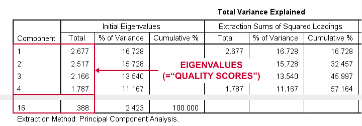
So what's a high Eigenvalue? A common rule of thumb is to select components whose Eigenvalues are at least 1. Applying this simple rule to the previous table answers our first research question: our 16 variables seem to measure 4 underlying factors.

This is because only our first 4 components have Eigenvalues of at least 1. The other components -having low quality scores- are not assumed to represent real traits underlying our 16 questions. Such components are considered “scree” as shown by the line chart below.

Factor Analysis Output II - Scree Plot

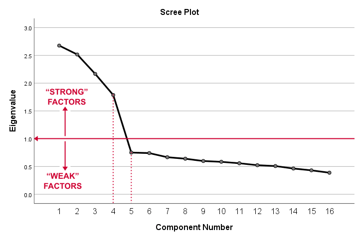
A scree plot visualizes the Eigenvalues (quality scores) we just saw. Again, we see that the first 4 components have Eigenvalues over 1. We consider these “strong factors”. After that -component 5 and onwards- the Eigenvalues drop off dramatically. The sharp drop between components 1-4 and components 5-16 strongly suggests that 4 factors underlie our questions.

Factor Analysis Output III - Communalities

So to what extent do our 4 underlying factors account for the variance of our 16 input variables? This is answered by the r square values which -for some really dumb reason- are called communalities in factor analysis.

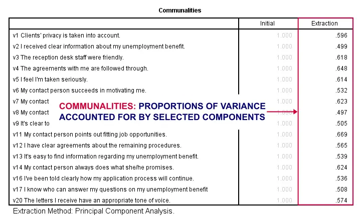
Right. So if we predict v1 from our 4 components by multiple regression, we'll find r square = 0.596 -which is v1’ s communality. Variables having low communalities -say lower than 0.40- don't contribute much to measuring the underlying factors.

You could consider removing such variables from the analysis. But keep in mind that doing so changes all results. So you'll need to rerun the entire analysis with one variable omitted. And then perhaps rerun it again with another variable left out.

If the scree plot justifies it, you could also consider selecting an additional component. But don't do this if it renders the (rotated) factor loading matrix less interpretable.

Factor Analysis Output IV - Component Matrix

Thus far, we concluded that our 16 variables probably measure 4 underlying factors. But which items measure which factors? The component matrix shows the Pearson correlations between the items and the components. For some dumb reason, these correlations are called factor loadings.

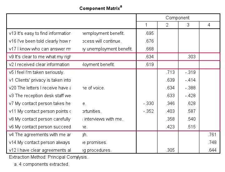
Ideally, we want each input variable to measure precisely one factor. Unfortunately, that's not the case here. For instance, v9 measures (correlates with) components 1 and 3. Worse even, v3 and v11 even measure components 1, 2 and 3 simultaneously. If a variable has more than 1 substantial factor loading, we call those cross loadings. And we don't like those. They complicate the interpretation of our factors.

The solution for this is rotation: we'll redistribute the factor loadings over the factors according to some mathematical rules that we'll leave to SPSS. This redefines what our factors represent. But that's ok. We hadn't looked into that yet anyway.

Now, there's different rotation methods but the most common one is the varimax rotation, short for “variable maximization. It tries to redistribute the factor loadings such that each variable measures precisely one factor -which is the ideal scenario for understanding our factors. And as we're about to see, our varimax rotation works perfectly for our data.

Factor Analysis Output V - Rotated Component Matrix

Our rotated component matrix (below) answers our second research question: “which variables measure which factors?”

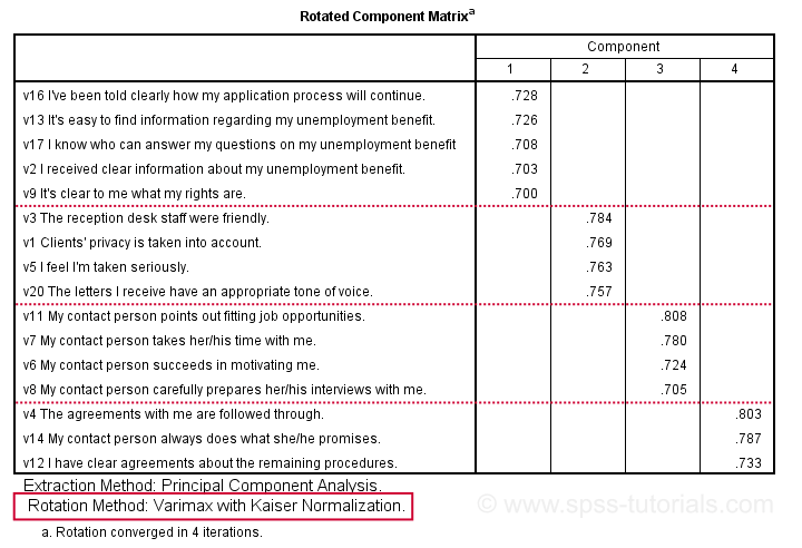
Our last research question is: “what do our factors represent?” Technically, a factor (or component) represents whatever its variables have in common. Our rotated component matrix (above) shows that our first component is measured by

• v17 - I know who can answer my questions on my unemployment benefit.
• v16 - I've been told clearly how my application process will continue.
• v13 - It's easy to find information regarding my unemployment benefit.
• v2 - I received clear information about my unemployment benefit.
• v9 - It's clear to me what my rights are.

Note that these variables all relate to the respondent receiving clear information. Therefore, we interpret component 1 as “clarity of information”. This is the underlying trait measured by v17, v16, v13, v2 and v9.

After interpreting all components in a similar fashion, we arrived at the following descriptions:

• Component 1 - “Clarity of information”
• Component 2 - “Decency and appropriateness”
• Component 3 - “Helpfulness contact person”
• Component 4 - “Reliability of agreements”

We'll set these as variable labels after actually adding the factor scores to our data.

Adding Factor Scores to Our Data

It's pretty common to add the actual factor scores to your data. They are often used as predictors in regression analysis or drivers in cluster analysis. SPSS FACTOR can add factor scores to your data but this is often a bad idea for 2 reasons:

• factor scores will only be added for cases without missing values on any of the input variables. We saw that this holds for only 149 of our 388 cases;
• factor scores are z-scores: their mean is 0 and their standard deviation is 1. This complicates their interpretation.

In many cases, a better idea is to compute factor scores as means over variables measuring similar factors. Such means tend to correlate almost perfectly with “real” factor scores but they don't suffer from the aforementioned problems. Note that you should only compute means over variables that have identical measurement scales.

It's also a good idea to inspect Cronbach’s alpha for each set of variables over which you'll compute a mean or a sum score. For our example, that would be 4 Cronbach's alphas for 4 factor scores but we'll skip that for now.

Computing and Labeling Factor Scores Syntax

Result

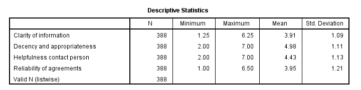
This descriptives table shows how we interpreted our factors. Because we computed them as means, they have the same 1 - 7 scales as our input variables. This allows us to conclude that

• “Decency and appropriateness” is rated best (roughly 5.0 out of 7 points) and
• “Clarity of information” is rated worst (roughly 3.9 out of 7 points).

Thanks for reading!

How to Run Levene’s Test in SPSS?

Levene’s test examines if 2+ populations all have
equal variances on some variable.

• Null Hypothesis
• Assumptions
• Levene’s test in SPSS
• Output
• Reporting

Levene’s Test - What Is It?

If we want to compare 2(+) groups on a quantitative variable, we usually want to know if they have equal mean scores. For finding out if that's the case, we often use

• an independent samples t-test for comparing 2 groups or
• a one-way ANOVA for comparing 3+ groups.

Both tests require the homogeneity (of variances) assumption: the population variances of the dependent variable must be equal within all groups. However, you don't always need this assumption:

• you don't need to meet the homogeneity assumption if the groups you're comparing have roughly equal sample sizes;
• you do need this assumption if your groups have sharply different sample sizes.

Now, we usually don't know our population variances but we do know our sample variances. And if these don't differ too much, then the population variances being equal seems credible.

But how do we know if our sample variances differ “too much”? Well, Levene’s test tells us precisely that.

Null Hypothesis

The null hypothesis for Levene’s test is that the groups we're comparing all have equal population variances. If this is true, we'll probably find slightly different variances in samples from these populations. However, very different sample variances suggest that the population variances weren't equal after all. In this case we'll reject the null hypothesis of equal population variances.

Levene’s Test - Assumptions

Levene’s test basically requires two assumptions:

• independent observations and
• the test variable is quantitative -that is, not nominal or ordinal.

Levene’s Test - Example

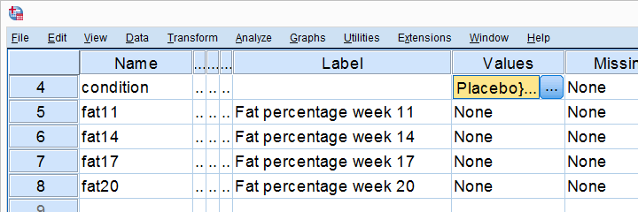
A fitness company wants to know if 2 supplements for stimulating body fat loss actually work. They test 2 supplements (a cortisol blocker and a thyroid booster) on 20 people each. An additional 40 people receive a placebo.

All 80 participants have body fat measurements at the start of the experiment (week 11) and weeks 14, 17 and 20. This results in fatloss-unequal.sav, part of which is shown below.

One approach to these data is comparing body fat percentages over the 3 groups (placebo, thyroid, cortisol) for each week separately.Perhaps a better approach to these data is using a single mixed ANOVA. Weeks would be the within-subjects factor and supplement would be the between-subjects factor. For now, we'll leave it as an exercise to the reader to carry this out. This can be done with an ANOVA for each of the 4 body fat measurements. However, since we've unequal sample sizes, we first need to make sure that our supplement groups have equal variances.

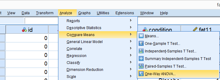
Running Levene’s test in SPSS

Several SPSS commands contain an option for running Levene’s test. The easiest way to go -especially for multiple variables- is the One-Way ANOVA dialog.This dialog was greatly improved in SPSS version 27 and now includes measures of effect size such as (partial) eta squared. So let's navigate to Analyze Compare Means One-Way ANOVA and fill out the dialog that pops up.

As shown below, the Homogeneity of variance test under Options refers to Levene’s test.

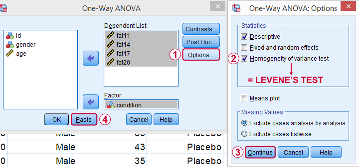
Clicking Paste results in the syntax below. Let's run it.

SPSS Levene’s Test Syntax Example

Output for Levene’s test

On running our syntax, we get several tables. The second -shown below- is the Test of Homogeneity of Variances. This holds the results of Levene’s test.

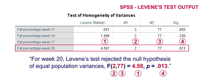
As a rule of thumb, we conclude that population variances are not equal if “Sig.” or p < .05. For the first 2 variables, p > .05: for fat percentage in weeks 11 and 14 we don't reject the null hypothesis of equal population variances.

For the last 2 variables, p < .05: for fat percentages in weeks 17 and 20, we reject the null hypothesis of equal population variances. So these 2 variables violate the homogeneity of variance assumption needed for an ANOVA.

Descriptive Statistics Output

Remember that we don't need equal population variances if we have roughly equal sample sizes. A sound way for evaluating if this holds is inspecting the Descriptives table in our output.

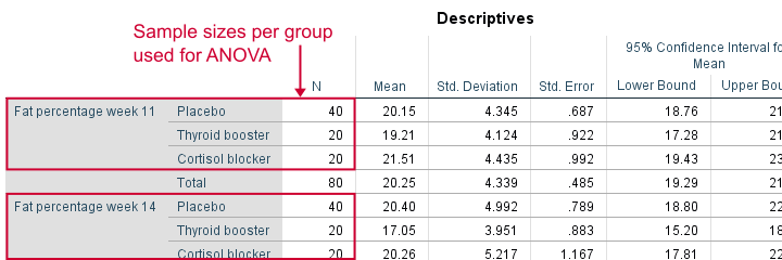
As we see, our ANOVA is based on sample sizes of 40, 20 and 20 for all 4 dependent variables. Because they're not (roughly) equal, we do need the homogeneity of variance assumption but it's not met by 2 variables.

In this case, we'll report alternative measures (Welch and Games-Howell) that don't require the homogeneity assumption. How to run and interpret these is covered in SPSS ANOVA - Levene’s Test “Significant”.

Reporting Levene’s test

Perhaps surprisingly, Levene’s test is technically an ANOVA as we'll explain here. We therefore report it like just a basic ANOVA too. So we'll write something like “Levene’s test showed that the variances for body fat percentage in week 20 were not equal, F(2,77) = 4.58, p = .013.”

Levene’s Test - How Does It Work?

Levene’s test works very simply: a larger variance means that -on average- the data values are “further away” from their mean. The figure below illustrates this: watch the histograms become “wider” as the variances increase.

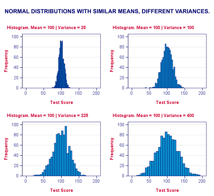
We therefore compute the absolute differences between all scores and their (group) means. The means of these absolute differences should be roughly equal over groups. So technically, Levene’s test is an ANOVA on the absolute difference scores. In other words: we run an ANOVA (on absolute differences) to find out if we can run an ANOVA (on our actual data).

If that confuses you, try running the syntax below. It does exactly what I just explained.

“Manual” Levene’s Test Syntax

Result

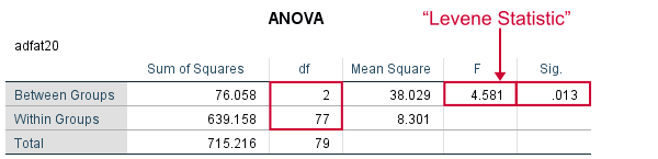
As we see, these ANOVA results are identical to Levene’s test in the previous output. I hope this clarifies why we report it as an ANOVA as well.

Thanks for reading!