SPSS COMPUTE – Simple Tutorial
SPSS COMPUTE command sets the data values for (possibly new) numeric variables and string variables. These values are usually a function (such as MEAN, SUM or something more advanced) of other variables.
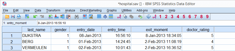
This tutorial walks you through doing just that. We'll use hospital.sav,a screenshot of which is shown below.
Before proceeding, we'll first set 6 as a user missing value for the last 5 variables. We'll do so by running the syntax below. missing values doctor_rating to facilities_rating (6).
SPSS COMPUTE Existing Numeric Variable
The simplest COMPUTE example is probably computing an already existing numeric variable. Say we'll add one point to facilities_rating because we feel our respondents were overly negative about it. The syntax below does just that. Note that COMPUTE is a transformation so we also run EXECUTE (“exe.”) in order to see the result.
compute facilities_rating = facilities_rating + 1.
exe.
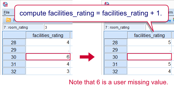
Note that 6 does not result in 7. This is because 6 is a user missing value and it's used in a basic numeric function.
SPSS COMPUTE New Numeric Variable
If the variable that's computed doesn't exit yet, SPSS will create it as a numeric variable having an f format. One of the implications is that we can't directly COMPUTE new string variables but we'll get to that in a minute. We first compute the mean over our 5 ratings but only for cases having at least 3 valid values. Note how this is easily accomplished by using the dot operator.
compute mean_score = mean.3(doctor_rating to facilities_rating).
exe.
SPSS COMPUTE Existing String Variable
In normal language, COMPUTE usually refers to operations on numbers. In SPSS, however, COMPUTE is used for setting the values of string variables as well. Keep in mind here that you can't use numeric functions on string variables or vice versa. The example below converts surname_prefix to lower case.
compute surname_prefix = lower(surname_prefix).
exe.
SPSS COMPUTE New String Variable
SPSS can compute only existing string variables. For new string variables, we must first create new (empty) variables with the STRING command. After doing so, we can set their values with COMPUTE. Like so, the syntax below creates full_name by concatenating the respondents' name components.
string full_name(a25).
*2. COMPUTE full_name with CONCAT and RTRIM.
compute full_name = concat(rtrim(first_name),' ',rtrim(surname_prefix),' ',rtrim(last_name)).
exe.
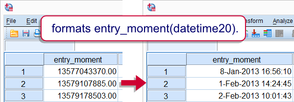
SPSS COMPUTE Date, Time and Datetime Variables
COMPUTE can be used for creating new date variables, time variables and datetime variables. This is because these are all numeric variables. However, new numeric variables always have an f format, which is usually not suitable for the aforementioned variables. The way to go here is to first computing the variables by using date functions or basic numeric functions. After doing so, use FORMATS for displaying their values appropriately. The syntax below gives an example.
compute entry_moment = entry_date + entry_time.
exe.
*2. Show datetime values (in seconds) as normal dates with times.
formats entry_moment(datetime20).
SPSS CROSSTABS – Simple Tutorial & Examples
SPSS CROSSTABS produces contingency tables: frequencies for one variable for each value of another variable separately. If assumptions are met, a chi-square test may follow to test whether an association between the variables is statistically significant. This tutorial, however, aims at quickly walking through the main options for CROSSTABS.
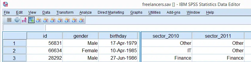
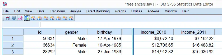
We'll use freelancers.sav throughout this tutorial as a test data file.
SPSS CROSSTABS - Minimal Specification
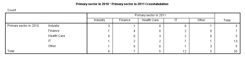
The syntax below demonstrates the simplest possible CROSSTABS command. It generates a table with the frequencies for sector_2010 for each value in sector_2011 separately. The screenshot below shows the result.
crosstabs sector_2010 by sector_2011.
SPSS CROSSTABS - CELLS Subcommand
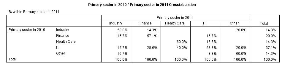
By default, CROSSTABS shows only frequencies (counts). However, the association between variables usually become more visible by displaying row or column percentages. They can be obtained by adding a CELLS subcommand.
Note that multiple cell contents may be chosen simultaneously; the second example below includes both column percentages and frequencies. Specifying ALL on the CELLS subcommand gives a complete overview of the options.
crosstabs sector_2010 by sector_2011/cells column.
*2. Crosstabs with both frequencies and column percentages in cells.
crosstabs sector_2010 by sector_2011/cells count column.
SPSS CROSSTABS - Multiway Tables
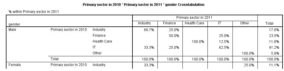
Multiway tables result from including more than one BY clause in CROSSTABS. Like so, the syntax below produces frequencies of sector_2011 for each combination of gender and sector_2010 separately. The following screenshot shows (part of) the result.
crosstabs sector_2010 by sector_2011 by gender
/cells column.
SPSS CROSSTABS - Multiple Tables, Similar Columns
Multiple tables with the same column variable but different row variables can be generated by a single CROSSTABS command; simply specify multiple variable names (possibly using TO) before the BY keyword. The syntax below gives an example.
crosstabs sector_2011 to sector_2014 by sector_2010.
SPSS CROSSTABS - Multiple Tables, Similar Rows
Multiple variables being specified after the BY keyword results in multiple tables with different column variables but the same row variable.
crosstabs sector_2010 by sector_2011 to sector_2014.
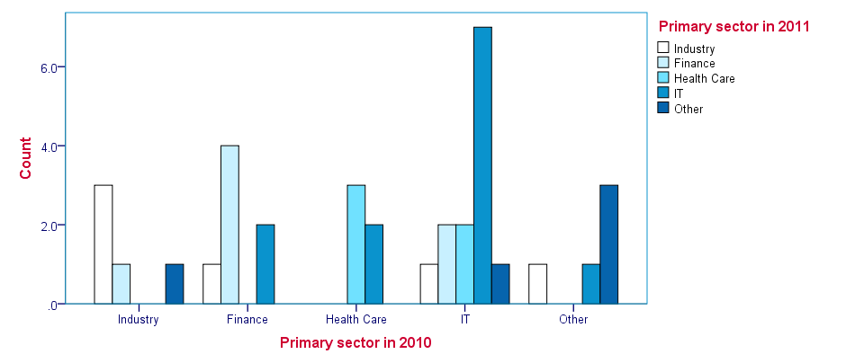
SPSS CROSSTABS - BARCHART Subcommand
Clustered barcharts can be obtained from CROSSTABS by simply adding a BARCHART subcommand as shown below. However, we prefer to generate such charts via GRAPH because it allows us to set appropriate titles for our charts.
Charts resulting from either option can be styled with an SPSS Chart Template (.sgt) file, which we used for the following screenshot.
crosstabs sector_2010 by sector_2011
/cells column
/barchart.
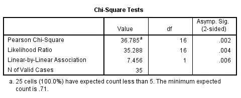
SPSS CROSSTABS - STATISTICS Subcommand
As mentioned in the introduction of this tutorial, CROSSTABS offers a chi-square test for evaluating the statistical significance of an association among the variables involved. It's obtained by specifying CHISQ on the STATISTICS subcommand.
Do keep in mind that SPSS happily produces test results even if their statistical assumptions don't hold, in which case such results may be wildly incorrect.
Besides the chi-square test statistic, many other statistics are available. For a full overview, specify ALL on the STATISTICS subcommand or consult the command syntax reference.
crosstabs sector_2010 by sector_2011
/cells column
/statistics chisq.
SPSS CORRELATIONS – Beginners Tutorial
Also see Pearson Correlations - Quick Introduction.
SPSS CORRELATIONS creates tables with Pearson correlations and their underlying N’s and p-values. For Spearman rank correlations and Kendall’s tau, use NONPAR-CORR. Both commands can be pasted from
![]()
![]() .
.
This tutorial quickly walks through the main options. We'll use freelancers.sav throughout and we encourage you to download it and follow along with the examples.
User Missing Values
Before running any correlations, we'll first specify all values of one million dollars or more as user missing values for income_2010 through income_2014.Inspecting their histograms (also see FREQUENCIES) shows that this is necessary indeed; some extreme values are present in these variables and failing to detect them will have a huge impact on our correlations. We'll do so by running the following line of syntax: missing values income_2010 to income_2014 (1e6 thru hi). Note that “1e6” is a shorthand for a 1 with 6 zeroes, hence one million.
SPSS CORRELATIONS - Basic Use
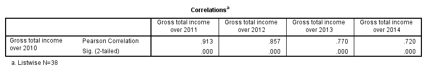
The syntax below shows the simplest way to run a standard correlation matrix. Note that due to the table structure, all correlations between different variables are shown twice.
By default, SPSS uses pairwise deletion of missing values here; each correlation (between two variables) uses all cases having valid values these two variables. This is why N varies from 38 through 40 in the screenshot below.
correlations income_2010 to income_2014.
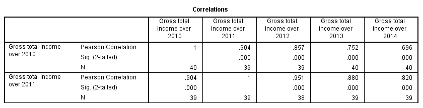
Keep in mind here that p-values are always shown, regardless of whether their underlying statistical assumptions are met or not. Oddly, SPSS CORRELATIONS doesn't offer any way to suppress them. However, SPSS Correlations in APA Format offers a super easy tool for doing so anyway.
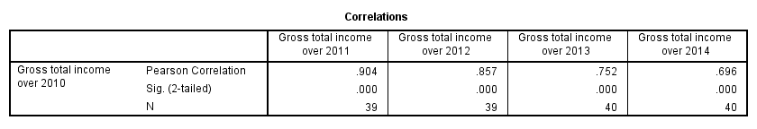
SPSS CORRELATIONS - WITH Keyword
By default, SPSS CORRELATIONS produces full correlation matrices. A little known trick to avoid this is using a WITH clause as demonstrated below. The resulting table is shown in the following screenshot.
correlations income_2010 with income_2011 to income_2014.
SPSS CORRELATIONS - MISSING Subcommand
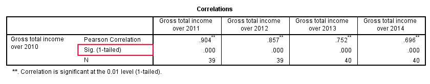
Instead of the aforementioned pairwise deletion of missing values, listwise deletion is accomplished by specifying it in a MISSING subcommand.An alternative here is identifying cases with missing values by using NMISS. Next, use FILTER to exclude them from the analysis. Listwise deletion doesn't actually delete anything but excludes from analysis all cases having one or more missing values on any of the variables involved.
Keep in mind that listwise deletion may seriously reduce your sample size if many variables and missing values are involved. Note in the next screenshot that the table structure is slightly altered when listwise deletion is used.
correlations income_2010 to income_2014
/missing listwise.
SPSS CORRELATIONS - PRINT Subcommand
By default, SPSS CORRELATIONS shows two-sided p-values. Although frowned upon by many statisticians, one-sided p-values are obtained by specifying ONETAIL on a PRINT subcommand as shown below.
Statistically significant correlations are flagged by specifying NOSIG (no, not SIG) on a PRINT subcommand.
correlations income_2010 with income_2011 to income_2014
/print nosig onetail.
SPSS CORRELATIONS - Notes
More options for SPSS CORRELATIONS are described in the command syntax reference. This tutorial deliberately skipped some of them such as inclusion of user missing values and capturing correlation matrices with the MATRIX subcommand. We did so due to doubts regarding their usefulness.
Thanks for reading!
SPSS Custom Dialogs – Quick Introduction
SPSS custom dialogs are extensions of SPSS’ point-click menu, officially known as the GUI (“graphical user interface”).
 SPSS Custom Dialogs in Menu
Custom dialogs are kept in files with the .spd file extension. After installing a custom dialog file, it will appear in the menu just like an SPSS' built-in command. The difference, however, is that SPSS users can build and share custom dialogs themselves, which isn't as difficult as it may seem.
SPSS Tutorials offers freely downloadable custom dialogs under Tools. Custom dialogs were introduced to SPSS in version 17.
Installing SPSS Custom Dialogs
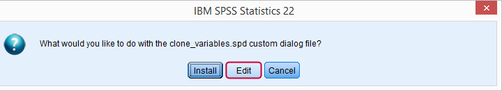
Option 1: the easiest way to install a custom dialog is simply double clicking the .spd file. A dialog window will pop up and ask you whether you'd like to install or edit the custom dialog.
 SPSS Custom Dialog Installation
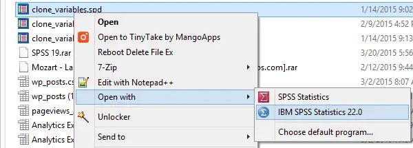
Option 2: If you have more than one SPSS version installed on your computer, right-click the .spd file and select the version in which you'd like to install it. Again, the installation window will pop up after doing so.
 SPSS Custom Dialogs in Menu
Option 3: alternatively, select ![]()
![]() .
.
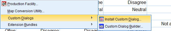 SPSS Custom Dialogs in Menu
Navigate to the .spd file. Clicking will launch the installer window.
SPSS Custom Dialogs in Menu
Navigate to the .spd file. Clicking will launch the installer window.
In some cases, SPSS may throw an Chi-Square Goodness-of-Fit Test - Simple Tutorial when you first install a custom dialog. Don't let this put you off. Troubleshooting this common error is not hard and needs to be done only once; subsequent custom dialogs will install more smoothly.
Uninstalling SPSS Custom Dialogs
Unfortunately, uninstalling SPSS custom dialogs is not straightforward and we strongly dislike the way this has been implemented in SPSS.
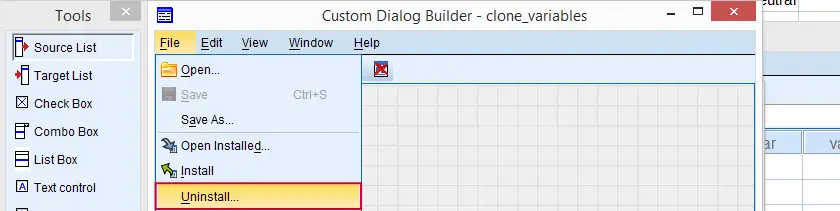
Option 1: open an .spd file as if you'd like to install it. This doesn't have to be the custom dialog you'd like to uninstall; any .spd file will do. Now, select as if you'd like to modify the custom dialog.
This will open an SPSS custom dialog builder window. You're probably not familiar with this window but don't panic, everything will be OK. Navigate to ![]() as shown below.
as shown below.
 SPSS Custom Dialog Builder Window
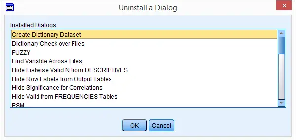
You now get a list of all custom dialogs installed (which is unrelated to the particular .spd file you used in order to arrive here). Select any custom dialog you'd like to uninstall. Clicking will uninstall it after asking whether you'd like to save the contents to a new .spd file. Close the custom dialog builder window without saving it when you're done.
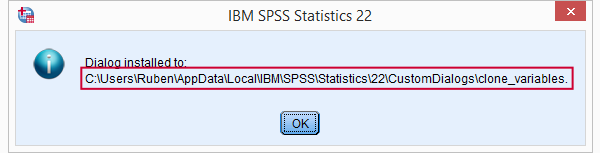
Option 2: (re)install any custom dialog. After doing so successfully, a window pops up that tells you where it was installed. Navigate to this folder and delete it entirely. Note: by default, some of these folders may be hidden in MS Windows.
SPSS Custom Dialogs - What are They?
Technically, a custom dialogs (.spd) files are archive files: zipped folders holding several smaller files. If you're curious, unzip one with 7 Zip to see what's inside.
A custom dialog's main element is the dialog window as the end user will see it. It may contain various elements such as plain text, variable selectors, text input and tick boxes.
 SPSS Custom Dialog Window
SPSS Custom Dialogs - How do they Work?
Underlying a custom dialog is syntax written by the author. It may contain placeholders that are replaced by whatever the end user specifies in the dialog window elements. This syntax, with the placeholders filled in, is run or pasted when or is clicked.
Note that many custom dialogs require the SPSS Python Essentials to be properly installed. If so, this should be clearly indicated on the dialog window itself and preferably in its user instructions as well.
Optionally, a Custom Dialog may contain a help file in HTML. If this is omitted, will be greyed out in the dialog window.
Clicking in one of our Tools will point your (default) web browser to the tutorial in which it was presented.
SPSS CD Command
A best practice in SPSS is to open and save all files with syntax. Like so, it can be easily seen which syntax was run on which data. One could use the syntax generated by for this but there's a much shorter and better option.
Disadvantages of the Default Syntax
- If you open and save several files, the total amount of syntax will be rather large. Especially if you write (rather than paste) your syntax, this may be a bit annoying even though you can copy-paste the folder specification
- If you move your project to a different folder, you'll need to correct all paths in order for them to be valid again
Shortening the Syntax
cd 'C:\Documents and Settings\Work\Projects 2012\December\Some Customer'.
*Open data file.
get file 'Survey data.sav'.
How Does it Work?
CD command sets a default directory. Whenever you open or save a file, it will be done from/to this directory. In case you're not sure what your default directory is, run
SHOW DIRECTORY.
In subsequent commands, you only have to type the file name, which is technically a relative path. Especially when you open or save multiple files, you'll need less syntax. More importantly, if you move your project to a different folder, you'll need to adjust only a single line of syntax (the cd command, that is). Especially when a project involves multiple syntax files, this may prove a major advantage, especially when combined with INSERT.Using Subfolders
Whenever you use relative rather than absolute paths, SPSS quietly prefixes them with the default directory. When you'd like to access a file in a subdirectory of the default directory, you can specify only the subdirectory and the file name.
For example, if your default directory is C:\project, then GET FILE 'data\data_file.sav'. will open data_file.sav from C:\project\data.
Final Notes
CD applies to all files such as
- data files (SPSS, Excel or any other format)
- SPSS output files
- SPSS syntax files when using INSERT
- SPSS chart templates (only in SPSS version 19 onwards)
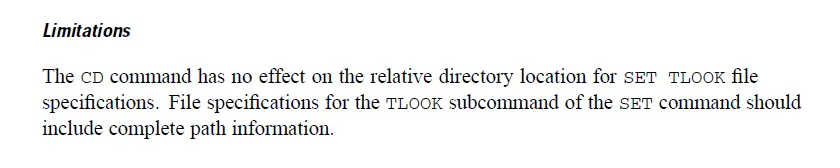
except tablelooks (“SET TLOOK ...”). I find this very annoying and I don't see why this hasn't fixed ages ago...
Thanks for reading!