SPSS FILTER – Quick & Simple Tutorial
SPSS FILTER temporarily excludes a selection of cases
from all data analyses.
For excluding cases from data editing, use DO IF or IF instead.
Quick Overview Contents
- SPSS Filtering Basics
- Example 1 - Exclude Cases with Many Missing Values
- Example 2 - Filter on 2 Variables
- Example 3 - Filter without Filter Variable
- Tip - Commands with Built-In Filters
- Warning - Data Editing with Filter
SPSS FILTER - Example Data
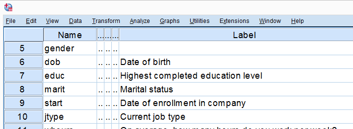
I'll use bank_clean.sav -partly shown below- for all examples in this tutorial. This file contains the data from a small bank employee survey. Feel free to download these data and rerun the examples yourself.
SPSS Filtering Basics
Filtering in SPSS usually involves 4 steps:
- create a filter variable;
- activate the filter variable;
- run one or many analyses -such as correlations, ANOVA or a chi-square test- with the filter variable in effect;
- deactivate the filter variable.
In theory, any variable can be used as a filter variable. After activating it, cases with
- zeroes,
- user missing values or
- system missing values
on the filter variable are excluded from all analyses until you deactivate the filter. For the sake of clarity, I recommend you only use filter variables containing 0 or 1 for each case. Enough theory. Let's put things into practice.
Example 1 - Exclude Cases with Many Missing Values
At the end of our data, we find 9 rating scales: q1 to q9. Perhaps we'd like to run a factor analysis on them or use them as predictors in regression analysis. In any case, we may want to exclude cases having many missing values on these variables. We'll first just count them by running the syntax below.
compute mis_1 = nmiss(q1 to q9).
*Apply variable label.
variable labels mis_1 'Number of missings on q1 to q9'.
*Check frequencies.
frequencies mis_1.
Result
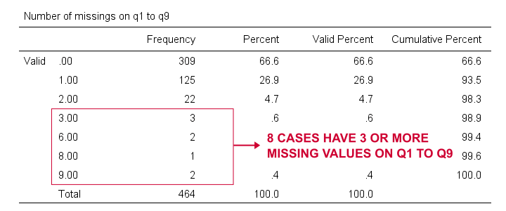
Based on this frequency distribution, we decided to exclude the 8 cases having 3 or more missing values on q1 to q9. We'll create our filter variable with a simple RECODE as shown below.
recode mis_1 (lo thru 2 = 1)(else = 0) into filt_1.
*Apply variable label.
variable labels filt_1 'Filter out cases with 3 or more missings on q1 to q9'.
*Activate filter variable.
filter by filt_1.
*Reinspect numbers of missings over q1 to q9.
frequencies mis_1.
Result
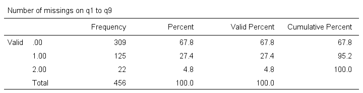
Note that SPSS now reports 456 instead of 464 cases. The 8 cases with 3 or more missing values are still in our data but they are excluded from all analyses. We can see why in data view as shown below.
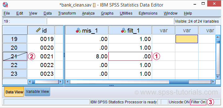
 Case 21 has 8 missing values on q1 to q9 and we recoded this into zero on our filter variable.
 The strikethrough its $casenum shows that case 21 is currently filtered out.
 The status bar confirms that a filter variable is in effect.
Finally, let's deactivate our filter by simply running
FILTER OFF.
We'll leave our filter variable filt_1 in the data. It won't bother us in any way.
The status bar confirms that a filter variable is in effect.
Finally, let's deactivate our filter by simply running
FILTER OFF.
We'll leave our filter variable filt_1 in the data. It won't bother us in any way.
Example 2 - Filter on 2 Variables
For some other analysis, we'd like to use only female respondents working in sales or marketing. A good starting point is running a very simple contingency table as shown below.
set tnumbers both.
*Show frequencies for job type per gender.
crosstabs gender by jtype.
Result
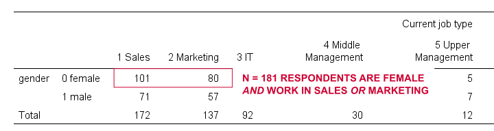
As our table shows, we've 181 female respondents working in either sales or marketing. We'll now create a new filter variable holding only zeroes. We'll then set it to 1 for our case selection with a simple IF command.
compute filt_2 = 0.
*Set filter to 1 for females in job types 1 and 2.
if(gender = 0 & jtype <= 2) filt_2 = 1.
*Apply variable label.
variable labels filt_2 'Filter in females working in sales and marketing'.
*Activate filter.
filter by filt_2.
*Confirm filter working properly.
crosstabs gender by jtype.
Rerunning our contingency table (not shown) confirms that SPSS now reports only 181 female cases working in marketing or sales. Also note that we now have 2 filter variables in our data and that's just fine but only 1 filter variable can be active at any time. Ok. Let's deactivate our new filter variable as well with FILTER OFF.
Example 3 - Filter without Filter Variable
Experienced SPSS users may know that
- TEMPORARY can “undo” some data editing that follow it and
- SELECT IF permanently deletes cases from your data.
By combining them you can circumvent the need for creating a filter variable but for 1 analysis at the time only. The example below shows just that: the first CROSSTABS is limited to a selection of cases but also rolls back our case deletion. The second CROSSTABS therefore includes all cases again.
temporary.
*Delete cases unless gender = 1 & jtype = 3.
select if (gender = 1 & jtype = 3).
*Crosstabs includes only males in IT and rolls back case selection.
crosstabs gender by jtype.
*Crosstabs includes all cases again.
crosstabs gender by jtype.
Tip - Commands with Built-In Filters
Something else you may want to know is that some commands have a built-in filter. These are
- REGRESSION,
- LOGISTIC REGRESSION,
- FACTOR and
- DISCRIMINANT.
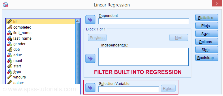
The dialog suggests you can filter cases -for this command only- based on just 1 variable. I suspect you can enter more complex conditions on the resulting /SELECT subcommand as well. I haven't tried it.
In any case, I think these built-in filters can be very handy and it kinda puzzles me they're only limited to the 4 aforementioned commands.
Warning - Data Editing with Filter
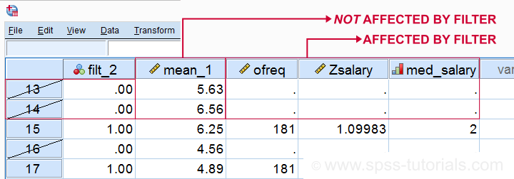
Most data editing in SPSS is unaffected by filtering. For example, computing means over variables -as shown below- affects all cases, regardless of whatever filter is active. We therefore need DO IF or IF to restrict this transformation to a selection of cases. However, an active filter does affect functions over cases. Some examples that we'll demonstrate below are
- adding a case count with AGGREGATE;
- computing z-scores for one or many variables;
- adding ranks, or percentiles with RANK.
SPSS Data Editing Affected by Filter Examples
filter by filt_2.
*Not affected by filter: add mean over q1 to q9 to data.
compute mean_1 = mean(q1 to q9).
execute.
*Affected by filter: add case count to data.
aggregate outfile * mode addvariables
/ofreq = n.
*Affected by filter: add z-scores salary to data..
descriptives salary
/save.
*Affected by filter: add median groups salary to data.
rank salary
/ntiles(2) into med_salary.
Result
Right. So that's pretty much all about filtering in SPSS. I hope you found this tutorial helpful and
Thanks for reading!
SPSS FREQUENCIES – Quick Tutorial
SPSS FREQUENCIES command can be used for much more than frequency tables: it's also the easiest way to obtain basic charts such as histograms and bar charts. On top of that, it provides us with percentiles and some other statistics. Plenty of reasons for taking a closer look at this ubiquitous SPSS command. We'll use employees.sav throughout this tutorial.
SPSS FREQUENCIES - Basic Table
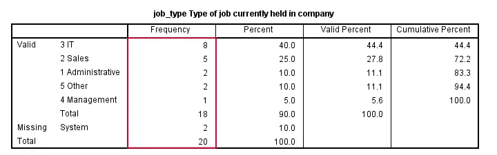
The most basic way to use FREQUENCIES is simply generating a frequency table. For example, the frequency table for job_type is obtained by running the following line of SPSS syntax: frequencies job_type.
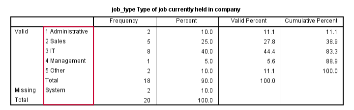
By default, the rows of this table are sorted ascendingly by value. Note that this may not be obvious when only value labels are displayed. We'll next take a look at different options for sorting the table rows.
SPSS FREQUENCIES - Sort Order
SPSS default sort order of ascendingly be value can be changed by adding a FORMAT subcommand. Possible values are AVALUE and DVALUE (ascending and descending values) or AFREQ and DFREQ (ascending and descending frequencies). For example, the syntax below sorts the rows from the value with highest frequency (yes, that's the mode) through the value with the lowest frequency.
frequencies job_type
/format dfreq.
SPSS FREQUENCIES - Bar Chart
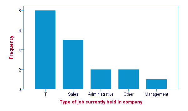
SPSS FREQUENCIES command is the easiest way to create one or more bar charts for categorical variables. Just add the BARCHART subcommand. Note that you can combine it with a sort order, resulting in the barchart bars being ordered from highest through lowest frequency as shown below.
frequencies job_type
/format dfreq
/barchart.
SPSS FREQUENCIES - Pie Chart
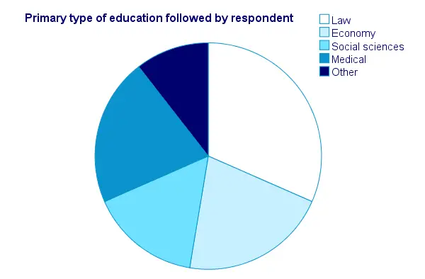
An alternative visualization for categorical variables is a pie chart. In order to generate it, simply add a PIECHART subcommand to FREQUENCIES. The syntax below creates a pie chart for education_type.
frequencies education_type
/piechart.
SPSS FREQUENCIES - Histogram
Frequency tables, bar charts and pie charts can all be used for both metric as well as categorical variables, including string variables. However, they are not useful for metric variables with many distinct values; in this case, tables get too many rows and graphs too many elements.
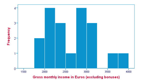
The ideal way to visualize such variables is a histogram, obtained by the HISTOGRAM subcommand. Apart from that, we can suppress frequency tables by specifying NOTABLE on the FORMAT subcommand. Like so, the syntax below generates a histogram for monthly_income.
frequencies monthly_income
/format notable
/histogram.
SPSS FREQUENCIES - Percentiles
SPSS FREQUENCIES provides a nice way to obtain percentiles: just add a PERCENTILES subcommand followed by the desired percentiles in parentheses. The syntax below gives an example. Keep in mind that percentiles are not meaningful for nominal variables.
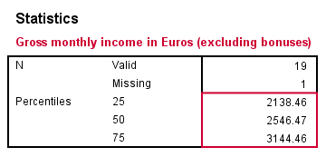
frequencies monthly_income
/format notable
/percentiles (25 50,75).
SPSS FREQUENCIES - Ntiles
Ntiles are easily obtained with SPSS FREQUENCIES: simply add the NTILES subcommand with the number of ntiles behind it in parentheses. If you want to assign cases to ntile groups, use RANK; it creates a new variable holding the ntile for each case on a given variable. Both options are shown in the syntax below.
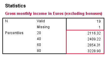
frequencies monthly_income
/format notable
/ntiles (5).
*2. Create monthly_income ntile group variable in data.
rank monthly_income/ntiles(5).
SPSS FREQUENCIES - Statistics
SPSS FREQUENCIES can compute all statistics obtained from DESCRIPTIVES plus the median and mode. Note that the statistics table from FREQUENCIES has a different layout with variables in columns and statistics in rows. For obtaining them, add a STATISTICS subcommand. Just as with DESCRIPTIVES, specifying the ALL keyword returns all available statistics.
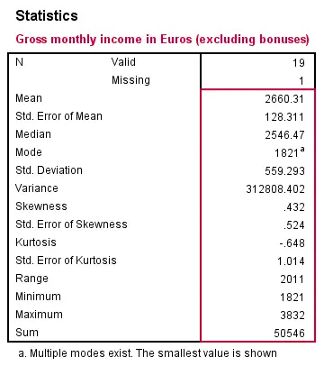
frequencies monthly_income
/format notable
/statistics all.
SPSS FREQUENCIES - Multiple Variables
Obviously, FREQUENCIES can be run for multiple variables, possibly using TO or ALL. If multiple types of output (frequency table, chart and so on) are generated, you can have them sorted by variable or output type by specifying VARIABLE or ANALYSIS on an ORDER subcommand.
frequencies education_type to job_type
/format dfreq
/barchart
/order variable.
*2. Sort output by output type (first tables for all variables, then charts for all variables).
frequencies education_type to job_type
/format dfreq
/barchart
/order analysis.
SPSS FORMATS – Set Display Format for Variables
SPSS FORMATS sets formats -decimal places, dates, percent signs and more- for numeric variables. Setting variable formats in SPSS does not change your actual data values. However, formats determine how your data are displayed -in the data viewer as well as the output window. Two main uses of FORMATS are
- increasing or decreasing the decimal places of standard numeric variables;
- displaying date, time and datetime values (consisting of numbers of seconds) as normal dates and times.
So let's try it and see how it works. All examples in this tutorial use employees.sav.
Setting Decimal Places
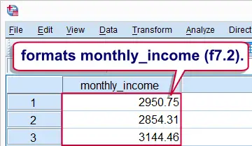
One of the main uses of FORMATS is setting decimal places for standard numeric variables by specifying their desired f formats. For example, we don't see any decimal places for monthly_income in data view except for the formula bar when we select a value (see screenshot).
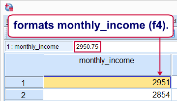
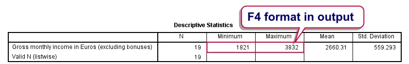
Its current format, F4, does not only hide all decimals in data view but affects some of the output as well. We can see this by running the following syntax: descriptives monthly_income.
SPSS FORMATS Syntax Example 1
We'll now set two decimal places for monthly_income and rerun the exact same DESCRIPTIVES command with the syntax below.
formats monthly_income(f7.2).
*2. Rerun descriptives.
descriptives monthly_income.
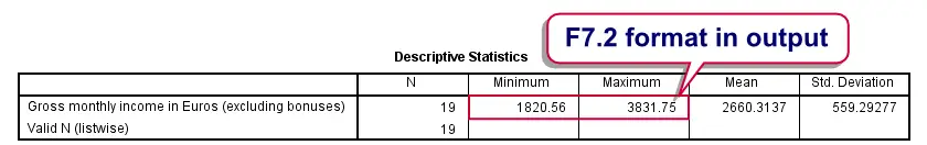
Note how all decimal places in the output table have increased by 2 by changing the variable's format. Apart from that, the F7.2 format also displays 2 decimal places in data view now (see next screenshot). Keep in mind that the actual values don't change in any way by running FORMATS.
Setting Date, Time and Datetime Formats
When new date variables, time variables and datetime variables are created, they may initially hold huge numbers that don't look like dates and time at all. These huge numbers are their actual values in numbers of seconds. These are only shown as normal dates and times after setting their formats appropriately. The syntax below demonstrates how to do so.
SPSS FORMATS Syntax Example 2
compute birthday_50 = datesum(date_of_birth,50,'years').
exe.
*2. Show numbers of seconds as normal date values.
formats birthday_50(date11).
The reason why this is usually necessary is that SPSS date, time and datetime variables are numeric variables. In SPSS, new numeric variables initially have an f format, usually F8.2. Those who really want to know can confirm this by running show format.
Multiple Variables
Formats can be set for multiple variables at once; after FORMATS, specify one or more variable names followed by their format. If desired, the command may continue with more variable names, again followed by their format. The syntax below gives an example.
SPSS FORMATS Syntax Example 3
formats education_type to experience_years(f2.1) monthly_income(dollar6) birthday_50(datetime20).