Kruskal-Wallis Test – Simple Tutorial

• Kruskal-Wallis Test Example
• Kruskal-Wallis Test Assumptions
• Kruskal-Wallis Test Formulas
• Kruskal-Wallis Post Hoc Tests
• APA Reporting a Kruskal-Wallis Test

A Kruskal-Wallis test tests if 3(+) populations have
equal mean ranks on some outcome variable. The figure below illustrates the basic idea.

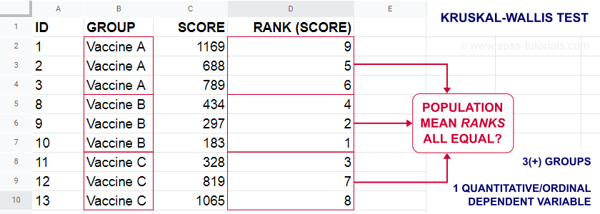
• First off, our scores are ranked ascendingly, regardless of group membership.
• Now, if scores are not related to group membership, then the average mean ranks should be roughly equal over groups.
• If these average mean ranks are very different in our sample, then some groups tend to have higher scores than other groups in our population as well: scores are related to group membership.

Kruskal-Wallis Test - Purposes

The Kruskal-Wallis test is a distribution free alternative for an ANOVA: we basically want to know if 3+ populations have equal means on some variable. However,

• ANOVA is not suitable if the dependent variable is ordinal;
• ANOVA requires the dependent variable to be normally distributed in each subpopulation, especially if sample sizes are small.

The Kruskal-Wallis test is a suitable alternative for ANOVA if sample sizes are small and/or the dependent variable is ordinal.

Kruskal-Wallis Test Example

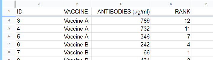
A hospital runs a quick pilot on 3 vaccines: they administer each to N = 5 participants. After a week, they measure the amount of antibodies in the participants’ blood. The data thus obtained are in this Googlesheet, partly shown below.

Now, we'd like to know if some vaccines trigger more antibodies than others in the underlying populations. Since antibodies is a quantitative variable, ANOVA seems the right choice here.

However, ANOVA requires antibodies to be normally distributed in each subpopulation. And due to our minimal sample sizes, we can't rely on the central limit theorem like we usually do (or should anyway). And on top of that, our sample sizes are too small to examine normality. Just the emphasize this point, the histograms for antibodies by group are shown below.

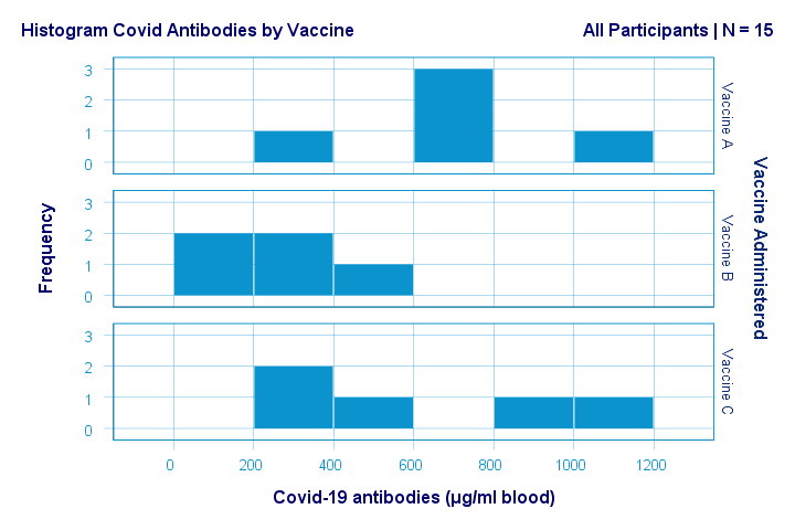
If anything, the bottom two histograms seem slightly positively skewed. This makes sense because the amount of antibodies has a lower bound of zero but no upper bound. However, speculations regarding the population distributions don't get any more serious than that.

A particularly bad idea here is trying to demonstrate normality by running

• a Shapiro-Wilk normality test and/or
• a Kolmogorov-Smirnov test.

Due to our tiny sample sizes, these tests are unlikely to reject the null hypothesis of normality. However, that's merely due to their lack of power and doesn't say anything about the population distributions. Put differently: a different null hypothesis (our variable following a uniform or Poisson distribution) would probably not be rejected either for the exact same data.

In short: ANOVA really requires normality for tiny sample sizes but we don't know if it holds. So we can't trust ANOVA results. And that's why we should use a Kruskal-Wallis test instead.

Kruskal-Wallis Test - Null Hypothesis

The null hypothesis for a Kruskal-Wallis test is that the mean ranks on some outcome variable
are equal across 3+ populations. Note that the outcome variable must be ordinal or quantitative in order for “mean ranks” to be meaningful.

Many textbooks propose an incorrect null hypothesis such as:

• some outcome variable has equal medians over 3+ populations or
• some outcome variable follows identical distributions over 3+ populations.

So why are these incorrect? Well, the Kruskal-Wallis formula uses only 2 statistics: ranks sums and the sample sizes on which they're based. It completely ignores everything else about the data -including medians and frequency distributions. Neither of these affect whether the null hypothesis is (not) rejected.

If that still doesn't convince you, we'll perhaps add some example data files to this tutorial. These illustrate that wildly different medians or frequency distributions don't always result in a “significant” Kruskal-Wallis test (or reversely).

Kruskal-Wallis Test Assumptions

A Kruskal-Wallis test requires 3 assumptions^1,5,8:

1. independent observations;
2. the dependent variable must be quantitative or ordinal;
3. sufficient sample sizes (say, each n_i ≥ 5) unless the exact significance level is computed.

Regarding the last assumption, exact p-values for the Kruskal-Wallis test can be computed. However, this is rarely done because it often requires very heavy computations. Some exact p-values are also found in Use of Ranks in One-Criterion Variance Analysis.

Instead, most software computes approximate (or “asymptotic”) p-values based on the chi-square distribution. This approximation is sufficiently accurate if the sample sizes are large enough. There's no real consensus with regard to required sample sizes: some authors¹ propose each n_i ≥ 4 while others⁶ suggest each n_i ≥ 6.

Kruskal-Wallis Test Formulas

First off, we rank the values on our dependent variable ascendingly, regardless of group membership. We did just that in this Googlesheet, partly shown below.

Next, we compute the sum over all ranks for each group separately.

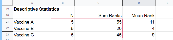
We then enter a) our samples sizes and b) our ranks sums into the following formula:

$$Kruskal\;Wallis\;H = \frac{12}{N(N + 1)}\sum\limits_{i = 1}^k\frac{R_i^2}{n_i} - 3(N + 1)$$

where

• \(N\) denotes the total sample size;
• \(k\) denotes the number of groups we're comparing;
• \(R_i\) denotes the rank sum for group \(i\);
• \(n_i\) denotes the sample size for group \(i\).

For our example, that'll be

$$Kruskal\;Wallis\;H = \frac{12}{15(15 + 1)}(\frac{55^2}{5}+\frac{20^2}{5}+\frac{45^2}{5}) - 3(15 + 1) =$$

$$Kruskal\;Wallis\;H = 0.05\cdot(605 + 80 + 405) - 48 = 6.50$$

\(H\) approximately follows a chi-square (written as χ²) distribution with

$$df = k - 1$$

degrees of freedom (\(df\)) for \(k\) groups. For our example,

$$df = 3 - 1 = 2$$

so our significance level is

$$\chi^2(2) = 6.50, p \approx 0.039.$$

The SPSS output for our example, shown below, confirms our calculations.

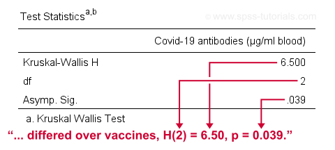
So what do we conclude now? Well, assuming alpha = 0.05, we reject our null hypothesis: the population mean ranks of antibodies are not equal among vaccines. In normal language, our 3 vaccines do not perform equally well. Judging from the mean ranks, it seems vaccine B performs worse than its competitors: its mean rank is lower and this means that it triggered fewer antibodies than the other vaccines.

Kruskal-Wallis Post Hoc Tests

Thus far, we concluded that the amounts of antibodies differ among our 3 vaccines. So precisely which vaccine differs from which vaccine? We'll compare each vaccine to each other vaccine for finding out. This procedure is generally known as running post-hoc tests.

In contrast to popular belief, Kruskal-Wallis post-hoc tests are not equivalent to Bonferroni corrected Mann-Whitney tests. Instead, each possible pair of groups is compared using the following formula:

$$Z_{kw} = \frac{\overline{R}_i - \overline{R}_j}{\sqrt{\frac{N(N + 1)}{12}(\frac{1}{n_i}+\frac{1}{n_j})}}$$

where

• our test statistic, \(Z_{kw}\), approximately follows a standard normal distribution;
• \(\overline R_i\) denotes the mean rank for group \(i\);
• \(N\) denotes the total sample size (including groups not used in this pairwise comparison);
• \(n_i\) denotes the sample size for group \(i\).

For comparing vaccines A and B, that'll be

$$Z_{kw} = \frac{11 - 4}{\sqrt{\frac{15(15 + 1)}{12}(\frac{1}{5}+\frac{1}{5})}} \approx 2.475 $$

$$P(|Z_{kw}| > 2.475) \approx 0.013$$

A Bonferroni correction is usually applied to this p-value because we're running multiple comparisons on (partly) the same observations. The number of pairwise comparisons for \(k\) groups is

$$N_{comp} = \frac{k (k - 1)}{2}$$

Therefore, the Bonferroni corrected p-value for our example is

$$P_{Bonf} = 0.013 \cdot \frac{3 (2 - 1)}{2} \approx 0.040$$

The screenshot from SPSS (below) confirms these findings.

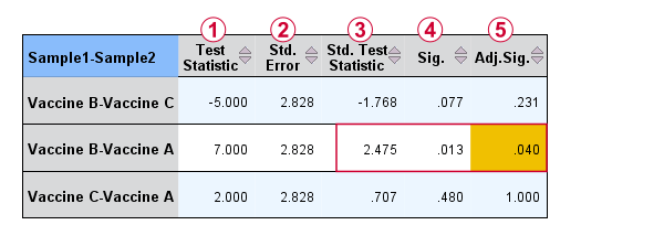
Oddly, the difference between mean ranks, \(\overline{R}_i - \overline{R}_j\), is denoted as “Test Statistic”.
The actual test statistic, \(Z_{kw}\) is denoted as “Std. Test Statistic”.

APA Reporting a Kruskal-Wallis Test

For APA reporting our example analysis, we could write something like “a Kruskal-Wallis test indicated that the amount of antibodies
differed over vaccines, H(2) = 6.50, p = 0.039.

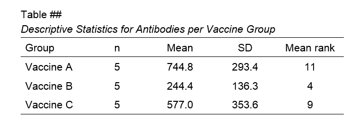
Although the APA doesn't mention it, we encourage reporting the mean ranks and perhaps some other descriptives statistics in a separate table as well.

Right, so that should do. If you've any questions or remarks, please throw me a comment below. Other than that:

Thanks for reading!

References

1. Van den Brink, W.P. & Koele, P. (2002). Statistiek, deel 3 [Statistics, part 3]. Amsterdam: Boom.
2. Warner, R.M. (2013). Applied Statistics (2nd. Edition). Thousand Oaks, CA: SAGE.
3. Agresti, A. & Franklin, C. (2014). Statistics. The Art & Science of Learning from Data. Essex: Pearson Education Limited.
4. Field, A. (2013). Discovering Statistics with IBM SPSS Statistics. Newbury Park, CA: Sage.
5. Howell, D.C. (2002). Statistical Methods for Psychology (5th ed.). Pacific Grove CA: Duxbury.
6. Siegel, S. & Castellan, N.J. (1989). Nonparametric Statistics for the Behavioral Sciences (2nd ed.). Singapore: McGraw-Hill.
7. Slotboom, A. (1987). Statistiek in woorden [Statistics in words]. Groningen: Wolters-Noordhoff.
8. Kruskal, W.H. & Wallis, W.A. (1952). Use of ranks in one-criterion variance analysis. Journal of the American Statistical Association, 47, 583-621.

SPSS – Kendall’s Concordance Coefficient W

Kendall’s Concordance Coefficient W is a number between 0 and 1
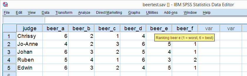
that indicates interrater agreement. So let's say we had 5 people rank 6 different beers as shown below. We obviously want to know which beer is best, right? But could we also quantify how much these raters agree with each other? Kendall’s W does just that.

Kendall’s W - Example

So let's take a really good look at our beer test results. The data -shown above- are in beertest.sav. For answering which beer was rated best, a Friedman test would be appropriate because our rankings are ordinal variables. A second question, however, is to what extent do all 5 judges agree on their beer rankings? If our judges don't agree at all which beers were best, then we can't possibly take their conclusions very seriously. Now, we could say that “our judges agreed to a large extent” but we'd like to be more precise and express the level of agreement in a single number. This number is known as Kendall’s Coefficient of Concordance W.^2,3

Kendall’s W - Basic Idea

Let's consider the 2 hypothetical situations depicted below: perfect agreement and perfect disagreement among our raters. I invite you to stare at it and think for a minute.

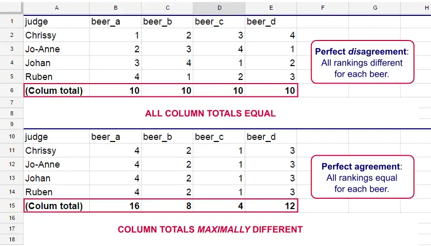
As we see, the extent to which raters agree is indicated by the extent to which the column totals differ. We can express the extent to which numbers differ as a number: the variance or standard deviation.
Kendall’s W is defined as

$$W = \frac{Variance\,over\,column\,totals}{Maximum\,possible\,variance\,over\,column\,totals}$$

As a result, Kendall’s W is always between 0 and 1. For instance, our perfect disagreement example has W = 0; because all column totals are equal, their variance is zero.
Our perfect agreement example has W = 1 because the variance among column totals is equal to the maximal possible variance. No matter how you rearrange the rankings, you can't possibly increase this variance any further. Don't believe me? Give it a go then.
So what about our actual beer data? We'll quickly find out with SPSS.

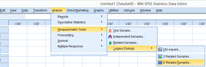
Kendall’s W in SPSS

We'll get Kendall’s W from SPSS’ Nonparametric Tests menu. The screenshots below walk you through.

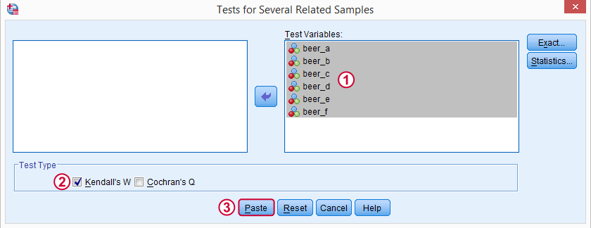
Note: SPSS thinks our rankings are nominal variables. This is because they contain few distinct values. Fortunately, this won't interfere with the current analysis. Completing these steps results in the syntax below.

Kendall’s W - Basic Syntax

Kendall’s W - Output

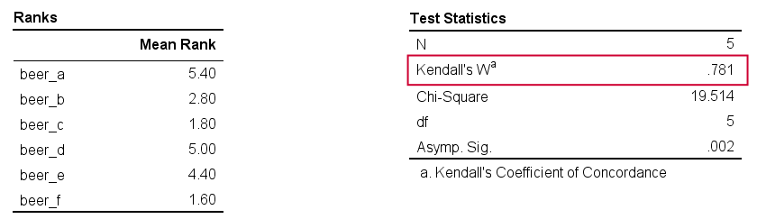
And there we have it: Kendall’s W = 0.78. Our beer judges agree with each other to a reasonable but not super high extent. Note that we also get a table with the (column) mean ranks that tells us which beer was rated most favorably.

Average Spearman Correlation over Judges

Another measure of concordance is the average over all possible Spearman correlations among all judges.¹ It can be calculated from Kendall’s W with the following formula

$$\overline{R}_s = {kW - 1 \over k - 1}$$

where \(\overline{R}_s\) denotes the average Spearman correlation and \(k\) the number of judges. For our example, this comes down to

$$\overline{R}_s = {5(0.781) - 1 \over 5 - 1} = 0.726$$

We'll verify this by running and averaging all possible Spearman correlations in SPSS. We'll leave that for a next tutorial, however, as doing so properly requires some highly unusual -but interesting- syntax.

Thank you for reading!

References

1. Howell, D.C. (2002). Statistical Methods for Psychology (5th ed.). Pacific Grove CA: Duxbury.
2. Slotboom, A. (1987). Statistiek in woorden [Statistics in words]. Groningen: Wolters-Noordhoff.
3. Van den Brink, W.P. & Koele, P. (2002). Statistiek, deel 3 [Statistics, part 3]. Amsterdam: Boom.

Kendall’s Tau – Simple Introduction

Kendall’s Tau is a number between -1 and +1
that indicates to what extent 2 variables are monotonously related.

• Kendall’s Tau - Formulas
• Kendall’s Tau - Exact Significance
• Kendall’s Tau - Confidence Intervals
• Kendall’s Tau versus Spearman Correlation
• Kendall’s Tau - Interpretation

Kendall’s Tau - What is It?

Kendall’s Tau is a correlation suitable for quantitative and ordinal variables. It indicates how strongly 2 variables are monotonously related: to which extent are high values on variable x are associated with
either high or low values on variable y? Like so, Kendall’s Tau serves the exact same purpose as the Spearman rank correlation. The reasoning behind the 2 measures, however, is different. Let's take a look at the example data shown below.

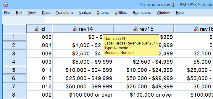
These data show yearly revenues over the years 2014 through 2018 for several companies. We'd like to know to what extent companies that did well in 2014 also did well in 2015. Note that we only have revenue categories and these are ordinal variables: we can rank them but we can't compute means, standard deviations or correlations over them.

Kendall’s Tau - Intersections Method

If we rank both years, we can inspect to what extent these ranks are different. A first step is to connect the 2014 and the 2015 ranks with lines as shown below.

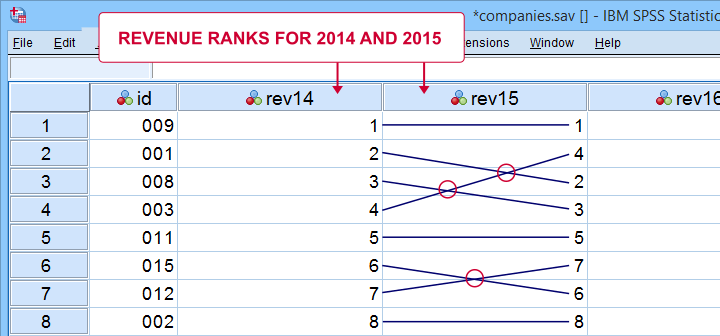
Our connection lines show 3 intersections. These are caused by the 2014 and 2015 rankings being slightly different. Note that the more the ranks differ, the more intersections we see:

• if 2 rankings are identical, we have zero intersections and
  
• if 2 rankings are exactly opposite, the number of intersections is

$$0.5\cdot n(n - 1)$$
This is the maximum number of intersections for \(n\) observations. Dividing the actual number of intersections by the maximum number of intersections is the basis for Kendall’s tau, denoted by \(\tau\) below.

$$\tau = 1 - \frac{2\cdot I}{0.5\cdot n(n - 1)}$$
where \(I\) is the number of intersections. For our example data with 3 intersections and 8 observations, this results in

$$\tau = 1 - \frac{2\cdot 3}{0.5\cdot 8(8 - 1)} =$$
$$\tau = 1 - \frac{6}{28} \approx 0.786$$

Since \(\tau\) runs from -1 to +1, \(\tau\) = 0.786 indicates a strong positive relation: higher revenue ranks in 2014 are associated with higher ranks in 2015.

Kendall’s Tau - Concordance Method

A second method to find Kendall’s Tau is to inspect all unique pairs of observations. We did so in this Googlesheet shown below.

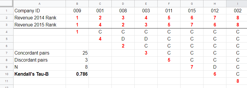
Starting at row 4, each 2015 rank is compared to all 2014 ranks to its right. If these are higher, we have concordant pairs of observations denoted by C. These indicate a positive relation.

However, 2015 ranks having larger 2014 ranks to their right indicate discordant pairs denoted by D. For instance, cell D5 is discordant because the 2014 rank (3) is smaller than the 2015 rank of 4. Discordant pairs indicate a negative relation.

Finally, Kendall’s Tau can be computed from the numbers of concordant and discordant pairs with $$\tau = \frac{n_c - n_d}{0.5\cdot n(n - 1)}$$

for our example with 3 discordant and 25 concordant pairs in 8 observations, this results in $$\tau = \frac{25 - 3}{0.5\cdot 8(8 - 1)} = $$
$$\tau = \frac{22}{28} \approx 0.786.$$
Note that C and D add up to the number of unique pairs of observations, \(0.5\cdot n(n - 1)\) which results 28 in our example. Keeping this in mind, you may see that

• \(\tau\) = -1 if all pairs are discordant;
• \(\tau\) = 0 if the numbers of concordant and discordant pairs are equal and
• \(\tau\) = 1 if all pairs are concordant.

Kendall’s Tau-B & Tau-C

Our first method for computing Kendall’s Tau only works if each company falls into a different revenue category. This holds for the 2014 and 2015 data. For 2017 and 2018, however, some companies fall into the same revenue categories. These variables are said to contain ties. Two modified formulas are used for this scenario:

• Kendall’s tau-b corrects for ties and
• Kendall’s tau-c ignores ties.

Simply “Kendall’s Tau” usually refers Kendall’s Tau-b. We won't discuss Kendall’s Tau-c as it's not often used anymore. In the absence of ties, both formulas yield identical results.

Kendall’s Tau - Formulas

So how could we deal with ties? First off, mean ranks are assigned to tied observations as in this Googlesheet shown below: companies 009 and 001 share the two lowest 2016 ranks so they are both ranked the mean of ranks 1 and 2, resulting in 1.5.

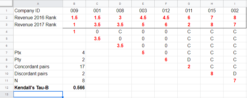
Second, pairs associated with tied 2016 observations are neither concordant nor discordant. Such pairs (columns B,C and E,F) receive a 0 rather than a C or a D. Third, 2017 ranks that have a 2017 tie to their right are also assigned 0. Like so, the 28 pairs in the example above result in

• 17 concordant pairs (C),
• 2 discordant pairs (D) and
• 9 inconclusive pairs (0).

For computing \(\tau_b\), ties on either variable result in a penalty computed as $$Pt = \Sigma{(t_i^2 - t_i)}$$
where \(t_i\) denotes the length of the \(i\)th tie for either variable. The 2016 ranks have 2 ties -both of length 2- resulting in $$Pt_{2016} = (2^2 - 2) + (2^2 - 2) = 4$$
Similarly, $$Pt_{2017} = (2^2 - 2) = 2$$

Finally, \(\tau_b\) is computed with $$\tau_b = \frac{2\cdot (C - D)}{\sqrt{n(n - 1) - Pt_x}\sqrt{n(n - 1) - Pt_y}}$$

For our example, this results in $$\tau_b = \frac{2\cdot (17 - 2)}{\sqrt{8(8 - 1) - 4}\sqrt{8(8 - 1) - 2}} =$$
$$\tau_b = \frac{30}{\sqrt{52}\sqrt{54}} \approx 0.566$$

Kendall’s Tau - Exact Significance

For small sample sizes of N ≤ 10, the exact significance level for \(\tau_b\) can be computed with a permutation test. The table below gives critical values for α = 0.05 and α = 0.01.

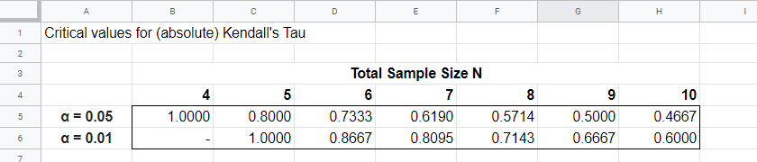
Our example calculation without ties resulted in \(\tau_b\) = 0.786 for 8 observations. Since \(|\tau_b|\) > 0.7143, p < 0.01: we reject the null hypothesis that \(\tau_b\) = 0 in the entire population. Basic conclusion: revenues over 2014 and 2015 are likely to have a positive monotonous relation in the entire population of companies.

The second example (with ties) resulted in \(\tau_b\) = 0.566 for 8 observations. Since \(|\tau_b|\) < 0.5714, p > 0.05. We retain the null hypothesis: our sample outcome is not unlikely if revenues over 2016 and 2017 are not monotonously related in the entire population.

Kendall’s Tau-B - Asymptotic Significance

For sample sizes of N > 10, $$z = \frac{3\tau_b\sqrt{n(n - 1)}}{\sqrt{2(2n + 5)}}$$

roughly follows a standard normal distribution. For example, if \(\tau_b\) = 0.500 based on N = 12 observations, $$z = \frac{3\cdot 0.500 \sqrt{12(11)}}{\sqrt{2(24 + 5)}} \approx 2.263$$

We can easily look up that \(p(|z| \gt 2.263) \approx 0.024\): we reject the null hypothesis that \(\tau_b\) = 0 in the population at α = 0.05 but not at α = 0.01.

Kendall’s Tau - Confidence Intervals

Confidence intervals for \(\tau_b\) are easily obtained from JASP. The screenshot below shows an output example.

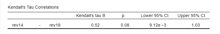
We presume that these confidence intervals require sample sizes of N > 10 but we couldn't find any reference on this.

Kendall’s Tau versus Spearman Correlation

Kendall’s Tau serves the exact same purpose as the Spearman rank correlation: both indicate to which extent 2 ordinal or quantitative variables are monotonously related. So which is better? Some general guidelines are that

1. the statistical properties -sampling distribution and standard error- are better known for Kendall’s Tau than for Spearman-correlations. Kendall’s Tau also converges to a normal distribution faster (that is, for smaller sample sizes). The consequence is that significance levels and confidence intervals for Kendall’s Tau tend to be more reliable than for Spearman correlations.
2. absolute values for Kendall’s Tau tend to be smaller than for Spearman correlations: when both are calculated on the same data, we typically see something like \(|\tau_b| \approx 0.7\cdot |R_s|\).
3. Kendall’s Tau typically has smaller standard errors than Spearman correlations. Combined with the previous point, the significance levels for Kendall’s Tau tend to be roughly equal to those for Spearman correlations.

In order to illustrate point 2, we computed Kendall’s Tau and Spearman correlations on 8 simulated variables, v1 through v8. The colors shown below are linearly related to the absolute values.

For basically all cells, the second line (Spearman correlation) is darker, indicating a larger absolute value. Also, \(|\tau_b| \approx 0.7\cdot |R_s|\) seems a rough but reasonable rule of thumb for most cells.

The significance levels for the same variables are shown below.

These colors show no clear pattern: sometimes Kendall’s Tau is “more significant” than Spearman’s rho and sometimes the reverse is true. Also note that the significance levels tend to be more similar than the actual correlations. Sadly, the positive skewness of these p-values results in limited dispersion among the colors.

Kendall’s Tau - Interpretation

• \(\tau_b\) = -1 indicates a perfect negative monotonous relation among 2 variables: a lower score on variable A is always associated with a higher score on variable B;
• \(\tau_b\) = 0 indicates no monotonous relation at all;
• \(\tau_b\) = 1 indicates a perfect positive monotonous relation: a lower score on variable A is always associated with a lower score on variable B.

The values of -1 and +1 can only be attained if both variables have equal numbers of distinct ranks, resulting in a square contingency table.

Furthermore, if 2 variables are independent, \(\tau_b\) = 0 but the reverse does not always hold: a curvilinear or other non monotonous relation may still exist.

We didn't find any rules of thumb for interpreting \(\tau_b\) as an effect size so we'll propose some:

• \(|\tau_b|\) = 0.07 indicates a weak association;
• \(|\tau_b|\) = 0.21 indicates a medium association;
• \(|\tau_b|\) = 0.35 indicates a strong association.

Kendall’s Tau-B in SPSS

The simplest option for obtaining Kendall’s Tau from SPSS is from the correlations dialog as shown below.

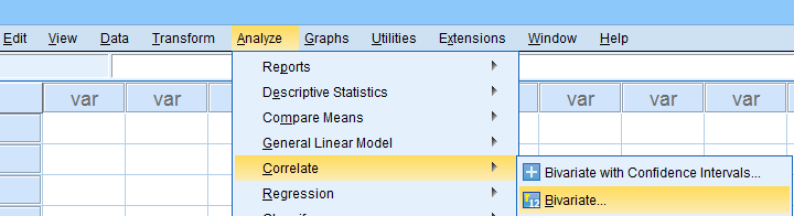
Alternatively (and faster), use simplified syntax such as

Thanks for reading!

Kurtosis – Quick Introduction

• Kurtosis Examples
• Kurtosis Formulas
• Kurtosis or Excess Kurtosis?
• Kurtosis Calculation Example
• Platykurtic, Mesokurtic and Leptokurtic

In statistics, kurtosis refers to the “peakedness”
of the distribution for a quantitative variable. What's meant by “peakedness” is best understood from the example histograms shown below.

Kurtosis Examples

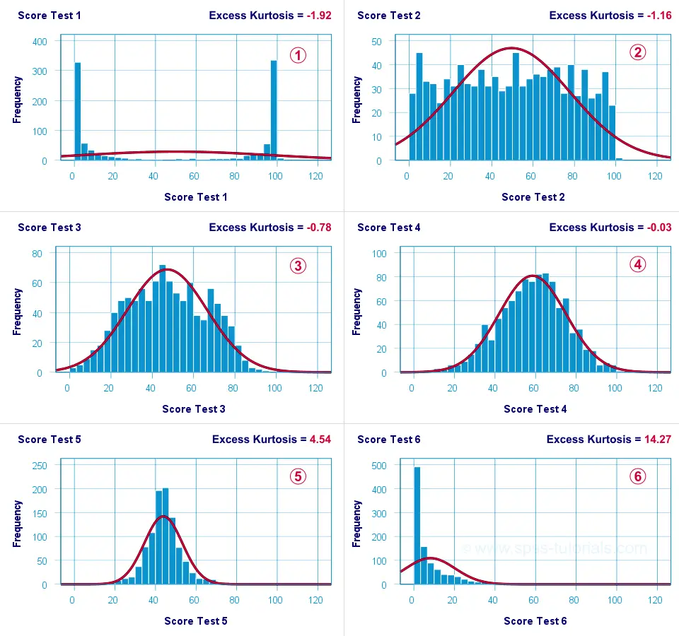
Test 4 is almost perfectly normally distributed. Its excess kurtosis is therefore close to 0.

The distribution for test 3 is somewhat “flatter” than the normal curve: the histogram bars are lower than the middle of the curve and higher towards its tails. Test 3 therefore has a negative excess kurtosis.

Test 5 is more “peaked” than the normal curve: its bars are higher than the peak of the curve and lower towards its tails. Therefore, test 5 has a positive excess kurtosis.

Test 2 roughly follows a uniform distribution. Because it's even flatter than test 3, it has a stronger negative excess kurtosis.

The strongest negative excess kurtosis is seen for test 1, which has a bimodal distribution.

Positive excess kurtosis is often seen for variables having strong (positive) skewness such as test 6.

So now that we've an idea what (excess) kurtosis means, let's see how it's computed.

Kurtosis Formulas

If your data contain an entire population rather than just a sample, the population kurtosis \(K_p\) is computed as

$$K_p = \frac{M_4}{M_2^2}$$

where \(M_2\) and \(M_4\) denote the second and fourth moments around the mean:

$$M_2 = \frac{\sum\limits_{i = 1}^N(X_i - \overline{X})^2}{N}$$

and

$$M_4 = \frac{\sum\limits_{i = 1}^N(X_i - \overline{X})^4}{N}$$

Note that \(M_2\) is simply the population-variance formula.

Kurtosis or Excess Kurtosis?

A normally distributed variable has a kurtosis of 3.0. Since this is undesirable, population excess kurtosis \(EK_p\) is defined as

$$EK_p = K_p - 3$$

so that excess kurtosis is 0.0 for a normally distributed variable.

Now, that's all fine. But what's not fine is that “kurtosis” refers to either kurtosis or excess kurtosis in standard textbooks and software packages without clarifying which of these two is reported.

Anyway.

Our formulas thus far only apply to data containing an entire population. If your data only contain a sample from some population -usually the case- then you'll want to compute sample excess kurtosis \(EK_s\) as

$$EK_s = ((N + 1) \cdot EK_p + 6) \cdot \frac{(N - 1)}{(N - 2) \cdot (N - 3)}$$

This formula results in “kurtosis” as reported by most software packages such as SPSS, Excel and Googlesheets. Finally, most text books suggest that the standard error for (excess) kurtosis \(SE_{eks}\) is computed as

$$SE_{eks} \approx \sqrt{\frac{24}{N}}$$

This approximation, however, is not accurate for small sample sizes. Therefore, software packages use a more complicated formula. I won't bother you with it.

Kurtosis Calculation Example

An example calculation for excess kurtosis is shown in this Googlesheet (read-only), partly shown below.

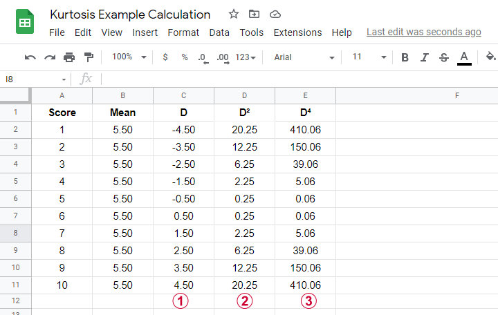
We computed excess kurtosis for scores 1 through 10. First off, we added their mean, M = 5.50. Next,

\(D\) denotes the difference scores (score - mean);
\(D^2\) are squared difference scores that are used for computing a variance;
\(D^4\) are difference scores raised to the fourth power.

As shown below, the remaining computations are fairly simple too.

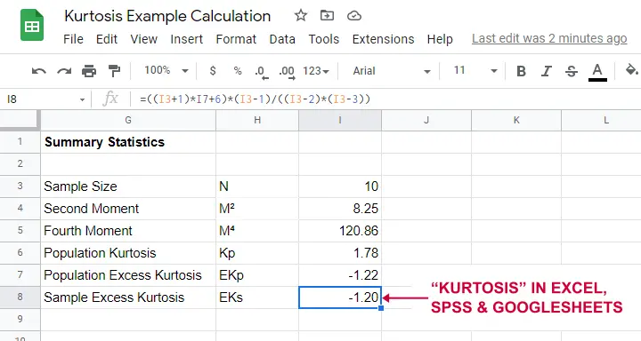
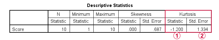
Note that the excess kurtosis = 1.20. The SPSS output shown below confirms this result.

Platykurtic, Mesokurtic & Leptokurtic

Some terminology related to excess kurtosis is that

• a variable having excess kurtosis < 0 is called platykurtic;
• a variable having excess kurtosis = 0 is called mesokurtic;
• a variable having excess kurtosis > 0 is called leptokurtic.

Our kurtosis examples illustrate what platykurtic, mesokurtic and leptokurtic distributions tend to look like.

Finding Kurtosis in Excel & SPSS

First off, “kurtosis” always refers to sample excess kurtosis in Excel, Googlesheets and SPSS. It's found in Excel and Googlesheets by using something like =KURT(A2:A11)

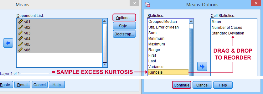
SPSS has many options for computing excess kurtosis but I personally prefer using Analyze Compare Means Means

As shown below, kurtosis can be selected from Options and dragged into the desired position.

Right, I think that's about it regarding (excess) kurtosis. If you've any questions or remarks, please throw me a comment below. Other than that:

thanks for reading!

SPSS Kolmogorov-Smirnov Test for Normality

An alternative normality test is the Shapiro-Wilk test.

• What is a Kolmogorov-Smirnov normality test?
• SPSS Kolmogorov-Smirnov test from NPAR TESTS
• SPSS Kolmogorov-Smirnov test from EXAMINE VARIABLES
• Reporting a Kolmogorov-Smirnov Test
• Wrong Results in SPSS?

What is a Kolmogorov-Smirnov normality test?

The Kolmogorov-Smirnov test examines if scores
are likely to follow some distribution in some population. For avoiding confusion, there's 2 Kolmogorov-Smirnov tests:

• there's the one sample Kolmogorov-Smirnov test for testing if a variable follows a given distribution in a population. This “given distribution” is usually -not always- the normal distribution, hence “Kolmogorov-Smirnov normality test”.
• there's also the (much less common) independent samples Kolmogorov-Smirnov test for testing if a variable has identical distributions in 2 populations.

In theory, “Kolmogorov-Smirnov test” could refer to either test (but usually refers to the one-sample Kolmogorov-Smirnov test) and had better be avoided. By the way, both Kolmogorov-Smirnov tests are present in SPSS.

Kolmogorov-Smirnov Test - Simple Example

So say I've a population of 1,000,000 people. I think their reaction times on some task are perfectly normally distributed. I sample 233 of these people and measure their reaction times.
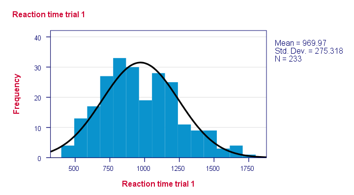
Now the observed frequency distribution of these will probably differ a bit -but not too much- from a normal distribution. So I run a histogram over observed reaction times and superimpose a normal distribution with the same mean and standard deviation. The result is shown below.

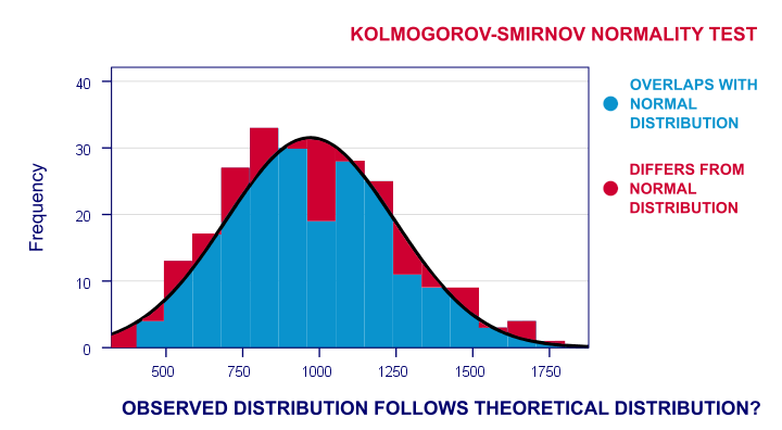
The frequency distribution of my scores doesn't entirely overlap with my normal curve. Now, I could calculate the percentage of cases that deviate from the normal curve -the percentage of red areas in the chart. This percentage is a test statistic: it expresses in a single number how much my data differ from my null hypothesis. So it indicates to what extent the observed scores deviate from a normal distribution.
Now, if my null hypothesis is true, then this deviation percentage should probably be quite small. That is, a small deviation has a high probability value or p-value.
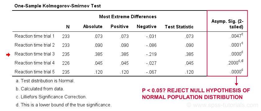
Reversely, a huge deviation percentage is very unlikely and suggests that my reaction times don't follow a normal distribution in the entire population. So a large deviation has a low p-value. As a rule of thumb, we reject the null hypothesis if p < 0.05. So if p < 0.05, we don't believe that our variable follows a normal distribution in our population.

Kolmogorov-Smirnov Test - Test Statistic

So that's the easiest way to understand how the Kolmogorov-Smirnov normality test works. Computationally, however, it works differently: it compares the observed versus the expected cumulative relative frequencies as shown below.

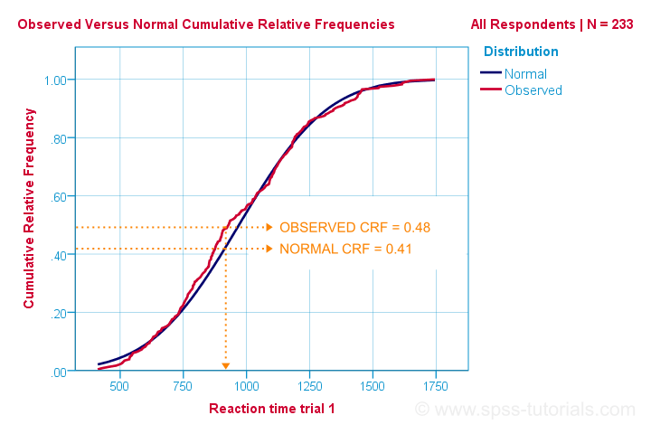
The Kolmogorov-Smirnov test uses the maximal absolute difference between these curves as its test statistic denoted by D. In this chart, the maximal absolute difference D is (0.48 - 0.41 =) 0.07 and it occurs at a reaction time of 960 milliseconds. Keep in mind that D = 0.07 as we'll encounter it in our SPSS output in a minute.

The Kolmogorov-Smirnov test in SPSS

There's 2 ways to run the test in SPSS:

• NPAR TESTS as found under Analyze Nonparametric Tests Legacy Dialogs 1-Sample K-S... is our method of choice because it creates nicely detailed output.
• EXAMINE VARIABLES from Analyze Descriptive Statistics Explore is an alternative. This command runs both the Kolmogorov-Smirnov test and the Shapiro-Wilk normality test.
  Note that EXAMINE VARIABLES uses listwise exclusion of missing values by default. So if I test 5 variables, my 5 tests only use cases which don't have any missings on any of these 5 variables. This is usually not what you want but we'll show how to avoid this.

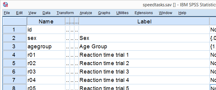
We'll demonstrate both methods using speedtasks.sav throughout, part of which is shown below.

Our main research question is which of the reaction time variables is likely
to be normally distributed in our population? These data are a textbook example of why you should thoroughly inspect your data before you start editing or analyzing them. Let's do just that and run some histograms from the syntax below.

Result

Note that some distributions do not look plausible at all. But which ones are likely to be normally distributed?

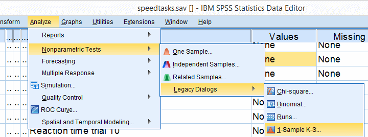
SPSS Kolmogorov-Smirnov test from NPAR TESTS

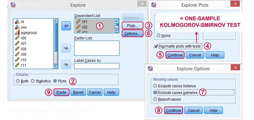
Our preferred option for running the Kolmogorov-Smirnov test is under Analyze Nonparametric Tests Legacy Dialogs 1-Sample K-S... as shown below.

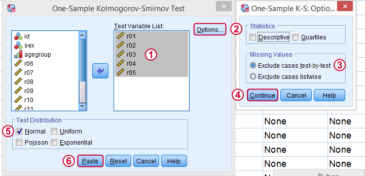
Next, we just fill out the dialog as shown below.

Clicking Paste results in the syntax below. Let's run it.

Kolmogorov-Smirnov Test Syntax from Nonparametric Tests

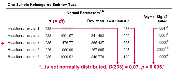
Results

First off, note that the test statistic for our first variable is 0.073 -just like we saw in our cumulative relative frequencies chart a bit earlier on. The chart holds the exact same data we just ran our test on so these results nicely converge.
Regarding our research question: only the reaction times for trial 4 seem to be normally distributed.

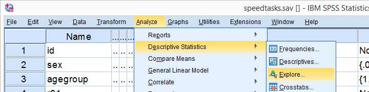
SPSS Kolmogorov-Smirnov test from EXAMINE VARIABLES

An alternative way to run the Kolmogorov-Smirnov test starts from Analyze Descriptive Statistics Explore as shown below.

Kolmogorov-Smirnov Test Syntax from Nonparametric Tests

Results

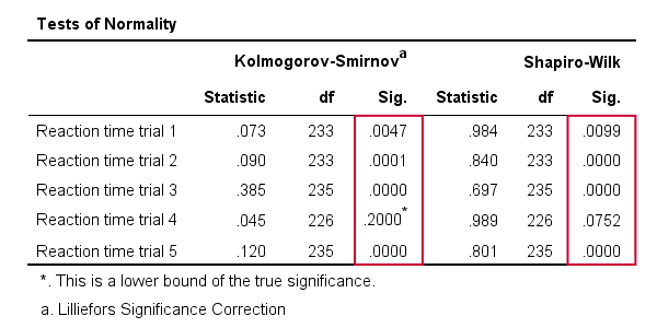
As a rule of thumb, we conclude that a variable is not normally distributed if “Sig.” < 0.05. So both the Kolmogorov-Smirnov test as well as the Shapiro-Wilk test results suggest that only Reaction time trial 4 follows a normal distribution in the entire population.
Further, note that the Kolmogorov-Smirnov test results are identical to those obtained from NPAR TESTS.

Reporting a Kolmogorov-Smirnov Test

For reporting our test results following APA guidelines, we'll write something like “a Kolmogorov-Smirnov test indicates that the reaction times on trial 1 do not follow a normal distribution, D(233) = 0.07, p = 0.005.” For additional variables, try and shorten this but make sure you include

• D (for “difference”), the Kolmogorov-Smirnov test statistic,
• df, the degrees of freedom (which is equal to N) and
• p, the statistical significance.

Wrong Results in SPSS?

If you're a student who just wants to pass a test, you can stop reading now. Just follow the steps we discussed so far and you'll be good.

Right, now let's run the exact same tests again in SPSS version 18 and take a look at the output.

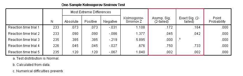
In this output, the exact p-values are included and -fortunately- they are very close to the asymptotic p-values. Less fortunately, though, the SPSS version 18 results are wildly different
from the SPSS version 24 results we reported thus far.
The reason seems to be the Lilliefors significance correction which is applied in newer SPSS versions. The result seems to be that the asymptotic significance levels differ much more from the exact significance than they did when the correction is not implied. This raises serious doubts regarding the correctness of the “Lilliefors results” -the default in newer SPSS versions.
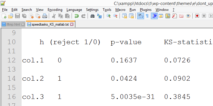
Converging evidence for this suggestion was gathered by my colleague Alwin Stegeman who reran all tests in Matlab. The Matlab results agree with the SPSS 18 results and -hence- not with the newer results.

Kolmogorov-Smirnov normality test - Limited Usefulness

The Kolmogorov-Smirnov test is often to test the normality assumption required by many statistical tests such as ANOVA, the t-test and many others. However, it is almost routinely overlooked that such tests are robust against a violation of this assumption if sample sizes are reasonable, say N ≥ 25.The underlying reason for this is the central limit theorem. Therefore, normality tests are only needed for small sample sizes if the aim is to satisfy the normality assumption.
Unfortunately, small sample sizes result in low statistical power for normality tests. This means that substantial deviations from normality will not result in statistical significance. The test says there's no deviation from normality while it's actually huge. In short, the situation in which normality tests are needed -small sample sizes- is also the situation in which they perform poorly.

Thanks for reading.