SPSS Z-Test for Independent Proportions Tutorial

• Z-Test - Assumptions
• SPSS Z-Tests Dialogs
• SPSS Z-Test Output
• SPSS Z-Tests - Strengths & Weaknesses
• APA Reporting Z-Tests

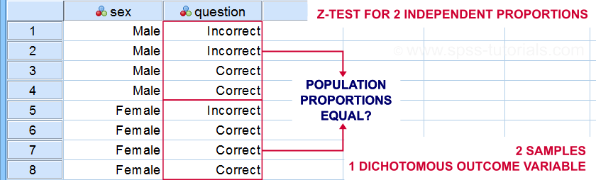
A z-test for independent proportions tests if 2 subpopulations
score similarly on a dichotomous variable. Example: are the proportions (or percentages) of correct answers equal between male and female students?

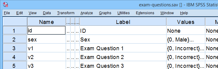
Although z-tests are widely used in the social sciences, they were only introduced in SPSS version 27. So let's see how to run them and interpret their output. We'll use exam-questions.sav -partly shown below- throughout this tutorial.

Now, before running the actual z-tests, we first need to make sure we meet their assumptions.

Z-Test - Assumptions

Z-tests for independent proportions require 2 assumptions:

• independent observations and
• sufficient sample sizes.

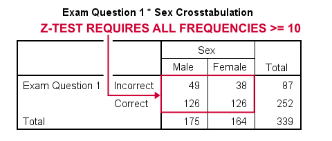
Regarding this second assumption, Agresti and Franklin (2014)² propose that both outcomes should occur at least 10 times in both samples. That is,

$$p_a n_a \ge 10, (1 - p_a) n_a \ge 10, p_b n_b \ge 10, (1 - p_b) n_b \ge 10$$

where

• \(n_a\) and \(n_b\) denote the sample sizes of groups a and b and
• \(p_a\) and \(p_b\) denote the proportions of “successes” in both groups.

Note that some other textbooks^3,4 suggest that smaller sample sizes may be sufficient. If you're not sure about meeting the sample sizes assumption, run a minimal CROSSTABS command as in crosstabs v1 to v5 by sex. As shown below, note that all 5 exam questions easily meet the sample sizes assumption.

For insufficient sample sizes, Agresti and Caffo (2000)¹ proposed a simple adjustment for computing confidence intervals: simply add one observation for each outcome to each group (4 observations in total) and proceed as usual with these adjusted sample sizes.

SPSS Z-Tests Dialogs

First off, let's navigate to Analyze Compare Means Independent-Samples Proportions and fill out the dialogs as shown below.

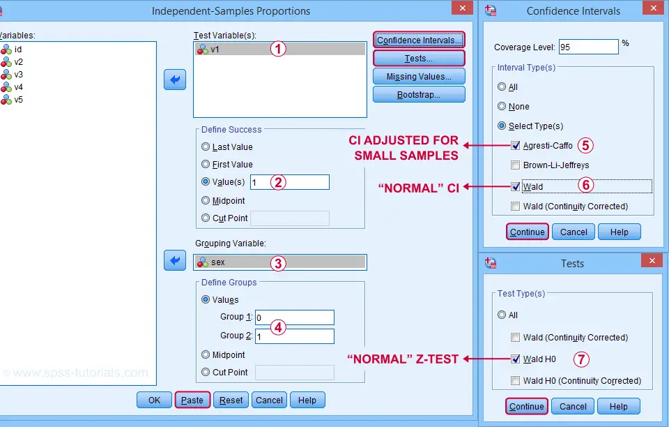
Clicking “Paste” results in the SPSS syntax below. Let's run it.

SPSS Z-Test Output

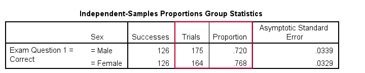
The first table shows the observed proportions for male and female students. Note that female students seem to perform somewhat better: a proportion of .768 (or 76.8%) answered correctly as compared to .720 for male students.

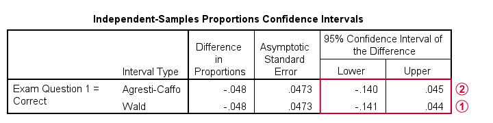
The second output table shows that the difference between our sample proportions is -.048.

The “normal” 95% confidence interval for this difference (denoted as Wald) is [-.141, .044]. Note that this CI encloses zero: male and female populations performing equally well is within the range of likely values.

I don't recommend reporting the Agresti-Caffo corrected CI unless your data don't meet the sample sizes assumption.

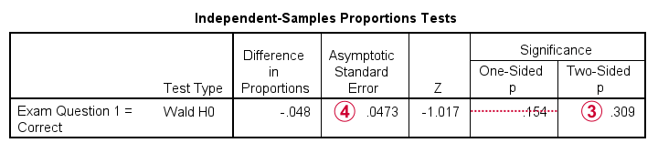
The third table shows the z-test results. First note that p(2-tailed) = .309. As a rule of thumb, we reject the null hypothesis if p < 0.05 which is not the case here. Conclusion: we do not reject the null hypothesis that the population difference is zero. That is: the sample difference of -.048 is not statistically significant.

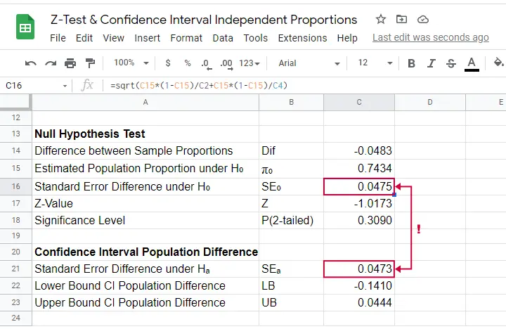
Finally, note that SPSS reports the wrong standard error for this test. The correct standard error is 0.0475 as computed in this Googlesheet (read-only) shown below.

SPSS Z-Tests - Strengths and Weaknesses

What's good about z-tests in SPSS is that

• you can analyze many dependent variables in one go;
• both the independent and dependent variables may be either string variables or numeric variables;We also tested SPSS z-tests on a mixture of string and numeric dependent variables. Although doing so is very awkward, the results were correct.
• many corrections -such as Agresti-Caffo- are available.

However, what I really don't like about SPSS z-tests is that

• no warning is issued if the sample sizes assumption isn't met;
• no effect size measures are available. Cohen’s H seems completely absent from SPSS and phi coefficients are available from CROSSTABS or CORRELATIONS;
• SPSS reports the wrong standard error for the actual z-test;
• z-tests and confidence intervals are reported in separate tables. I'd rather see these as different columns in a single table with one row per dependent variable.

APA Reporting Z-Tests

The APA guidelines don't explicitly mention how to report z-tests. However, it makes sense to report something like the difference between males and females
was not significant, z = -1.02, p(2-tailed) = .309. You should obviously report the actual proportions and sample sizes as well. If you analyzed multiple dependent variables, you may want to create a table showing

• both proportions being compared;
• the difference between the proportions and its confidence interval;
• z and p(2-tailed) for the null hypothesis of equal population proportions;
• some effect size measure.

References

1. Agresti, A & Caffo, B. (2000). Simple and Effective Confidence Intervals for Proportions and Differences of Proportions. The American Statistician, 54(4), 280-288.
2. Agresti, A. & Franklin, C. (2014). Statistics. The Art & Science of Learning from Data. Essex: Pearson Education Limited.
3. Twisk, J.W.R. (2016). Inleiding in de Toegepaste Biostatistiek [Introduction to Applied Biostatistics]. Houten: Bohn Stafleu van Loghum.
4. Van den Brink, W.P. & Koele, P. (2002). Statistiek, deel 3 [Statistics, part 3]. Amsterdam: Boom.

SPSS Median Test for 2 Independent Medians

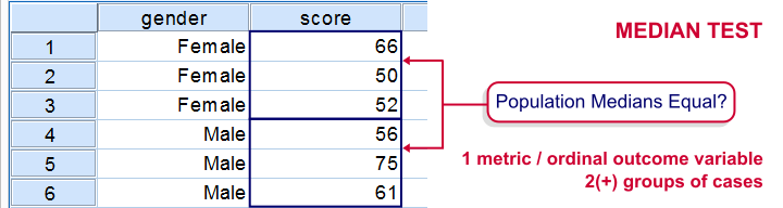
The median test for independent medians tests if two or more populations have equal medians on some variable. That is, we're comparing 2(+) groups of cases on 1 variable at a time.

Rating Car Commercials

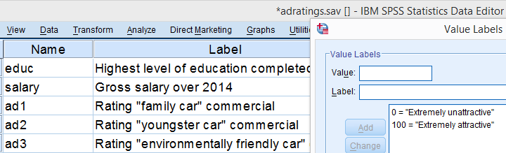
We'll demonstrate the median test on adratings.sav. This file holds data on 18 respondents who rated 3 different car commercials on attractiveness. A percent scale was used running from 0 (extremely unattractive commercial) through 100 (extremely attractive).

Median Test - Null Hypothesis

A marketeer wants to know if men rate the 3 commercials differently than women. After comparing the mean scores with a Mann-Whitney test, he also wants to know if the median scores are equal. A median test will answer the question by testing the null hypothesis that the population medians for men and women are equal for each rating variable.

Median Test - Assumptions

The median test makes only two assumptions:

• independent observations (or more precisely, independent and identically distributed variables);
• the test variable is ordinal or metric (that is, not nominal).

Quick Data Check

The adratings data don't hold any weird values or patterns. If you're analyzing any other data, make sure you always start with a data inspection. At the very least, run some histograms and check for missing values.

Median Test - Descriptives

Right, we're comparing 2 groups of cases on 3 rating variables. Let's first just take a look at the resulting 6 medians. The fastest way for doing so is running a basic MEANS command.

Result

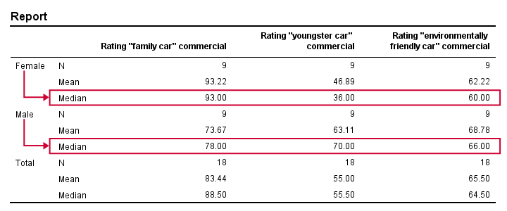
Very basically, the “family car” commercial was rated better by female respondents. Males were more attracted to the “youngster car” commercial. The “environmentally friendly car” commercial was rated roughly similarly by both genders -with regard to the medians anyway.
Now, keep in mind that this is just a small sample. If the population medians are exactly equal, then we'll probably find slightly different medians in our sample due to random sampling fluctuations. However, very different sample medians suggest that the population medians weren't equal after all. The median test tells us if equal population medians are credible, given our sample medians.

Median Test in SPSS

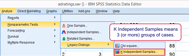
Usually, comparing 2 statistics is done with a different test than 3(+) statistics.For example, we use an independent samples t-test for 2 independent means and one-way ANOVA for 3(+) independent means. We use a paired samples t-test for 2 dependent means and repeated measures ANOVA for 3(+) dependent means. We use a McNemar test for 2 dependent proportions and a Cochran Q test for 3(+) dependent proportions. The median test is an exception because it's used for 2(+) independent medians. This is why we select K independent samples instead of 2 independent samples for comparing 2 medians.

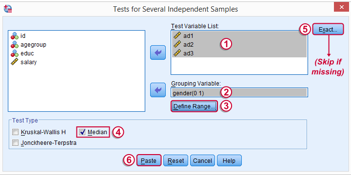
The Exact button may be absent, depending on your SPSS license. If it's present, fill it out as below.

SPSS Median Test Syntax

Completing these steps results in the syntax below (you'll have an extra line if you selected the exact test).

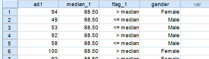
Median Test - How it Basically Works

Before inspecting our output, let's first take a look at how the test basically works for one variable.² The median test first computes a variable’s median, regardless of the groups we're comparing. Next, each case (row of data values) is flagged if its score > the pooled median. Finally, we'll see if scoring > the median is related to gender with a basic crosstab.You can pretty easily run these steps yourself with AGGREGATE, IF and CROSSTABS.

Median Test Output - Crosstabs

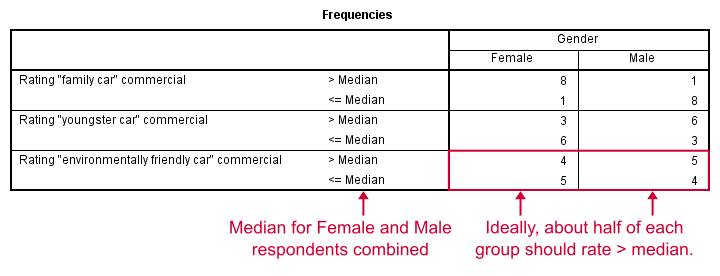
Note that these results are in line with the medians we ran earlier. The result for our “family car” commercial is particularly striking: 8 out of 9 respondents who score higher than the (pooled) median are female.

Median Test Output - Test Statistics

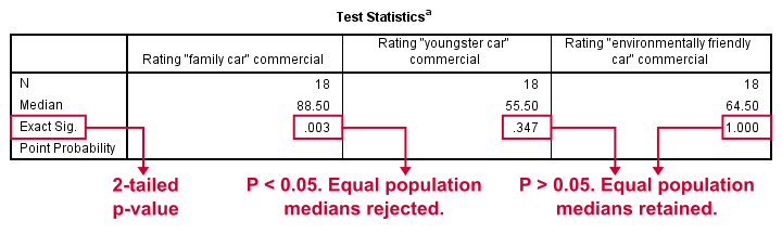
So are these normal outcomes if our population medians are equal across gender? For our first commercial, p = 0.003, indicating a chance of 3 in 1,000 of observing this outcome. Since p < 0.05, we conclude that the population medians are not equal for the “family car” commercial.
The other two commercials have p-values > 0.05 so these findings don't refute the null hypothesis of equal population medians.
So that's basically it for now. However, we would like to discuss the p-values into a little more detail for those who are interested.

Asymp. Sig.

In this example, we got exact p-values. However, when running this test on larger samples you may find “Asymp. Sig.” in your output. This is an approximate p-value based on the chi-square statistic and corresponding df (degrees of freedom). This approximation is sometimes used because the exact p-values are cumbersome to compute, especially for larger sample sizes.

Exact P-Values

So where do the exact p-values come from? How do they relate to the contingency tables we saw here? Well, the frequencies in the left upper cells follow a hypergeometric distribution.¹ Like so, the figure below shows where the second p-value of 0.347 comes from.

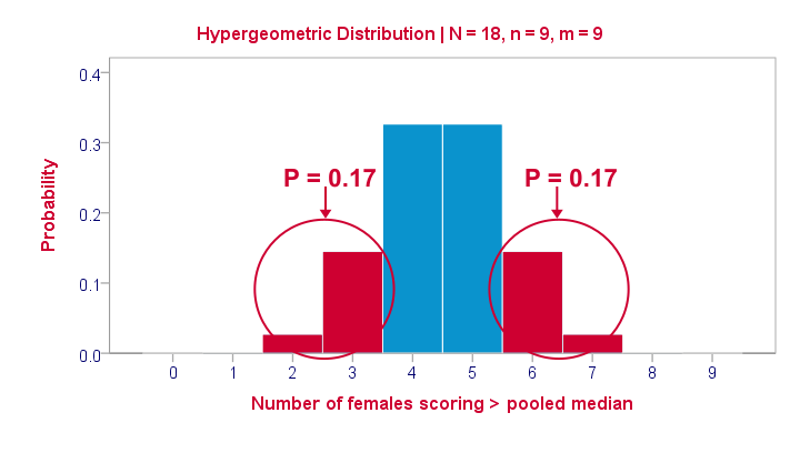
Under the null hypothesis -gender and scoring > the median are independent- the most likely outcome is 4 or 5, each with a probability around 0.33. The probability of 3 or fewer is roughly 0.17. This is our one-tailed p-value. Our two-tailed p-value takes into account the probability of 0.17 for finding a value of 6 or more because this would also contradict our null hypothesis.
The graph also illustrates why the two-tailed p-value for our third test is 1.000: the probability of 4 or fewer and 5 or more covers all possible outcomes. Regarding our first test, the probability of 1 or fewer and 8 or more is close to zero (precisely: 0.003).

Median Test with CROSSTABS

Right, so the previous figure explains how exact p-values are based on the hypergeometric distribution. This procedure is known as Fisher’s exact test and you may have seen it in SPSS CROSSTABS output when running a chi-square independence test. And -indeed- you can obtain the exact p-values for our independent medians test from CROSSTABS too. In fact, you can even compute them as a new variable in your data with compute p2 = 2* cdf.hyper(3,18,9,9).
execute. which returns 0.347, the p-value for our second commercial.

Thanks for reading!

References

1. Siegel, S. & Castellan, N.J. (1989). Nonparametric Statistics for the Behavioral Sciences (2nd ed.). Singapore: McGraw-Hill.
2. Van den Brink, W.P. & Koele, P. (2002). Statistiek, deel 3 [Statistics, part 3]. Amsterdam: Boom.

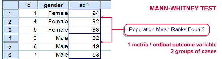
SPSS Mann-Whitney Test Tutorial

Introduction & Practice Data File

The Mann-Whitney test is an alternative for the independent samples t-test when the assumptions required by the latter aren't met by the data. The most common scenario is testing a non normally distributed outcome variable in a small sample (say, n < 25).Non normality isn't a serious issue in larger samples due to the central limit theorem.

The Mann-Whitney test is also known as the Wilcoxon test for independent samples -which shouldn't be confused with the Wilcoxon signed-ranks test for related samples.

Research Question

We'll use adratings.sav during this tutorial, a screenshot of which is shown above. These data contain the ratings of 3 car commercials by 18 respondents, balanced over gender and age category. Our research question is whether men and women judge our commercials similarly. For each commercial separately, our null hypothesis is: “the mean ratings of men and women are equal.”

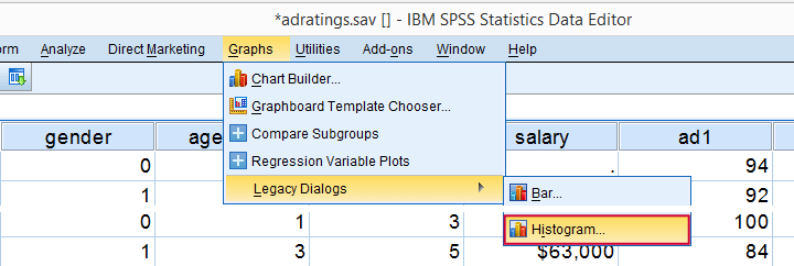
Quick Data Check - Split Histograms

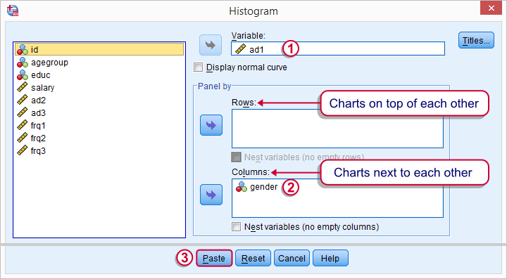
Before running any significance tests, let's first just inspect what our data look like in the first place. A great way for doing so is running some histograms. Since we're interested in differences between male and female respondents, let's split our histograms by gender. The screenshots below guide you through.

Split Histograms - Syntax

Using the menu results in the first block of syntax below. We copy-paste it twice, replace the variable name and run it.

Split Histograms - Results

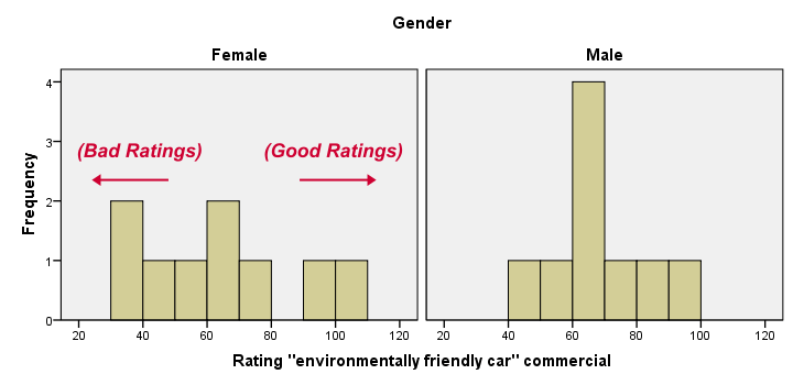
Most importantly, all results look plausible; we don't see any unusual values or patterns. Second, our outcome variables don't seem to be normally distributed and we've a total sample size of only n = 18. This argues against using a t-test for these data.
Finally, by taking a good look at the split histograms, you can already see which commercials are rated more favorably by male versus female respondents. But even if they're rated perfectly similarly by large populations of men and women, we'll still see some differences in small samples. Large sample differences, however, are unlikely if the null hypothesis -equal population means- is really true. We'll now find out if our sample differences are large enough for refuting this hypothesis.

SPSS Mann-Whitney Test - Menu

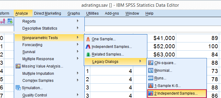
Depending on your SPSS license, you may or may not have the Exact submenu available. If you don't have it, just skip the step below.

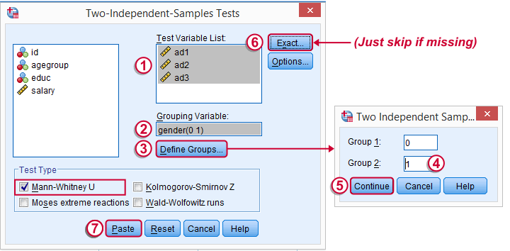
SPSS Mann-Whitney Test - Syntax

Note: selecting Exact results in an extra line of syntax (omitted below).

SPSS Mann-Whitney Test - Output Descriptive Statistics

The Mann-Whitney test basically replaces all scores with their rank numbers: 1, 2, 3 through 18 for 18 cases. Higher scores get higher rank numbers. If our grouping variable (gender) doesn't affect our ratings, then the mean ranks should be roughly equal for men and women.

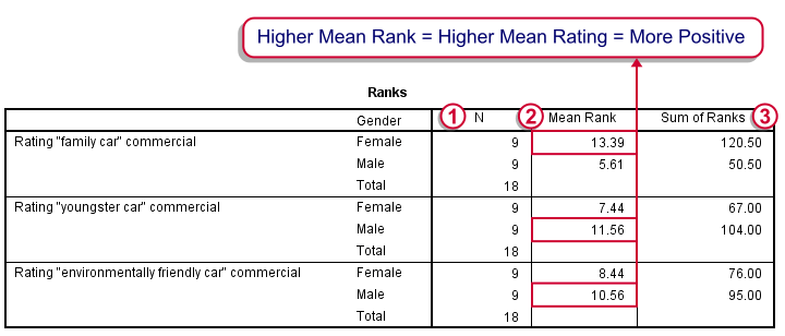
Our first commercial (“Family car”) shows the largest difference in mean ranks between male and female respondents: females seem much more enthusiastic about it. The reverse pattern -but much weaker- is observed for the other two commercials.

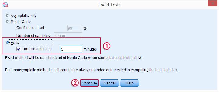
SPSS Mann-Whitney Test - Output Significance Tests

Some of the output shown below may be absent depending on your SPSS license and the sample size: for n = 40 or fewer cases, you'll always get some exact results.

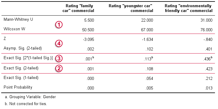
Mann-Whitney U and Wilcoxon W are our test statistics; they summarize the difference in mean rank numbers in a single number.Note that Wilcoxon W corresponds to the smallest sum of rank numbers from the previous table.
We prefer reporting Exact Sig. (2-tailed): the exact p-value corrected for ties.
Second best is Exact Sig. [2*(1-tailed Sig.)], the exact p-value but not corrected for ties.
For larger sample sizes, our test statistics are roughly normally distributed. An approximate (or “Asymptotic”) p-value is based on the standard normal distribution. The z-score and p-value reported by SPSS are calculated without applying the necessary continuity correction, resulting in some (minor) inaccuracy.

SPSS Mann-Whitney Test - Conclusions

Like we just saw, SPSS Mann-Whitney test output may include up to 3 different 2-sided p-values. Fortunately, they all lead to the same conclusion if we follow the convention of rejecting the null hypothesis if p < 0.05: Women rated the “Family Car” commercial more favorably than men (p = 0.001). The other two commercials didn't show a gender difference (p > 0.10). The p-value of 0.001 indicates a probability of 1 in 1,000: if the populations of men and women rate this commercial similarly, then we've a 1 in 1,000 chance of finding the large difference we observe in our sample. Presumably, the populations of men and women don't rate it similarly after all.

So that's about it. Thanks for reading and feel free to leave a comment below!