SPSS Factor Analysis – Beginners Tutorial
- What is Factor Analysis?
- Quick Data Checks
- Running Factor Analysis in SPSS
- SPSS Factor Analysis Output
- Adding Factor Scores to Our Data
What is Factor Analysis?
Factor analysis examines which underlying factors are measured
by a (large) number of observed variables.
Such “underlying factors” are often variables that are difficult to measure such as IQ, depression or extraversion. For measuring these, we often try to write multiple questions that -at least partially- reflect such factors. The basic idea is illustrated below.
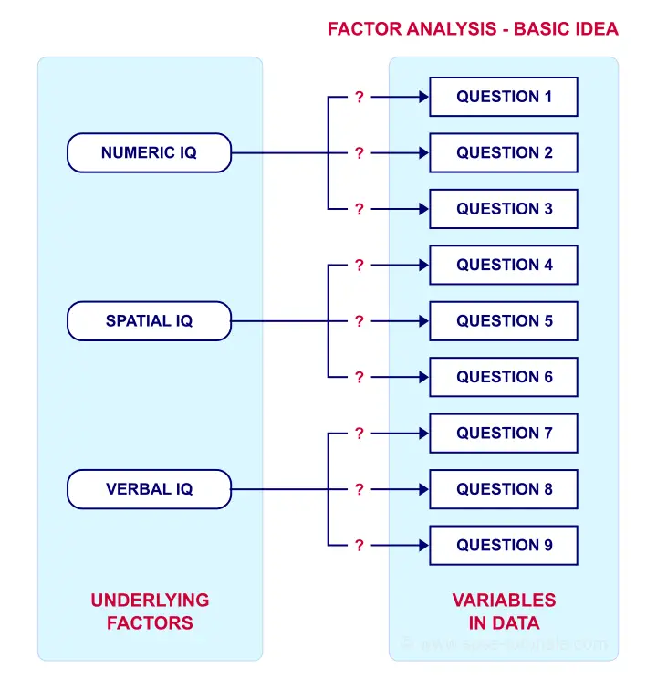
Now, if questions 1, 2 and 3 all measure numeric IQ, then the Pearson correlations among these items should be substantial: respondents with high numeric IQ will typically score high on all 3 questions and reversely.
The same reasoning goes for questions 4, 5 and 6: if they really measure “the same thing” they'll probably correlate highly.
However, questions 1 and 4 -measuring possibly unrelated traits- will not necessarily correlate. So if my factor model is correct, I could expect the correlations to follow a pattern as shown below.
Confirmatory Factor Analysis
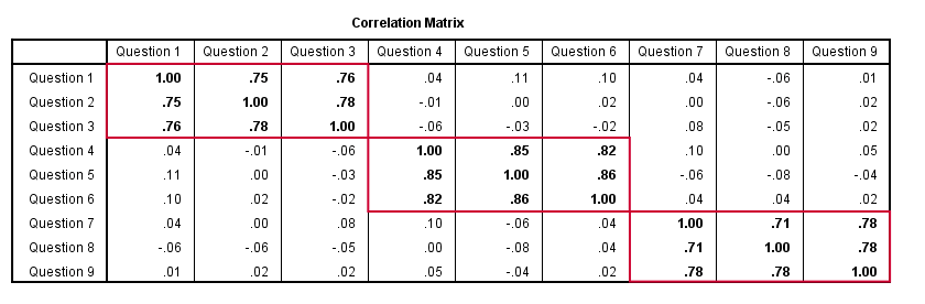
Right, so after measuring questions 1 through 9 on a simple random sample of respondents, I computed this correlation matrix. Now I could ask my software if these correlations are likely, given my theoretical factor model. In this case, I'm trying to confirm a model by fitting it to my data. This is known as “confirmatory factor analysis”.
SPSS does not include confirmatory factor analysis but those who are interested could take a look at AMOS.
Exploratory Factor Analysis
But what if I don't have a clue which -or even how many- factors are represented by my data? Well, in this case, I'll ask my software to suggest some model given my correlation matrix. That is, I'll explore the data (hence, “exploratory factor analysis”). The simplest possible explanation of how it works is that
the software tries to find groups of variables
that are highly intercorrelated.
Each such group probably represents an underlying common factor. There's different mathematical approaches to accomplishing this but the most common one is principal components analysis or PCA. We'll walk you through with an example.
Research Questions and Data
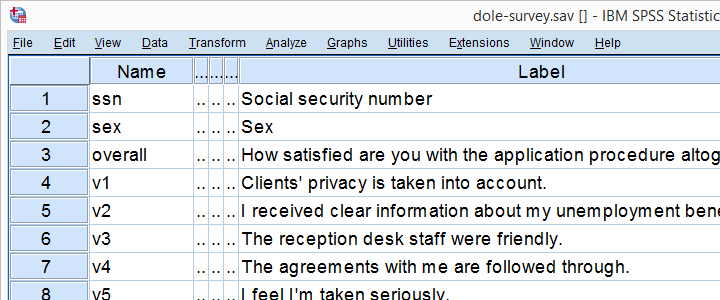
A survey was held among 388 applicants for unemployment benefits. The data thus collected are in dole-survey.sav, part of which is shown below.
The survey included 16 questions on client satisfaction. We think these measure a smaller number of underlying satisfaction factors but we've no clue about a model. So our research questions for this analysis are:
- how many factors are measured by our 16 questions?
- which questions measure similar factors?
- which satisfaction aspects are represented by which factors?
Quick Data Checks
Now let's first make sure we have an idea of what our data basically look like. We'll inspect the frequency distributions with corresponding bar charts for our 16 variables by running the syntax below.
set
tnumbers both /* show values and value labels in output tables */
tvars both /* show variable names but not labels in output tables */
ovars names. /* show variable names but not labels in output outline */
*Basic frequency tables with bar charts.
frequencies v1 to v20
/barchart.
Result
This very minimal data check gives us quite some important insights into our data:
- All frequency distributions look plausible. We don't see anything weird in our data.
- All variables are
 positively coded: higher values always indicate more positive sentiments.
 - All variables have
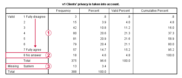
 a value 8 (“No answer”) which we need to set as a user missing value.
 - All variables have some
 system missing values too but the extent of missingness isn't too bad.
A somewhat annoying flaw here is that we don't see variable names for our bar charts in the output outline.
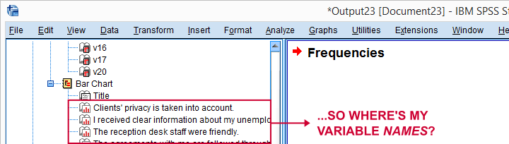
If we see something unusual in a chart, we don't easily see which variable to address. But in this example -fortunately- our charts all look fine.
So let's now set our missing values and run some quick descriptive statistics with the syntax below.
missing values v1 to v20 (8).
*Inspect valid N for each variable.
descriptives v1 to v20.
Result
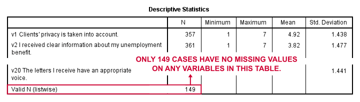
Note that none of our variables have many -more than some 10%- missing values. However, only 149 of our 388 respondents have zero missing values on the entire set of variables. This is very important to be aware of as we'll see in a minute.
Running Factor Analysis in SPSS
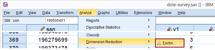
Let's now navigate to
![]()
![]() as shown below.
as shown below.
In the dialog that opens, we have a ton of options. For a “standard analysis”, we'll select the ones shown below. If you don't want to go through all dialogs, you can also replicate our analysis from the syntax below.
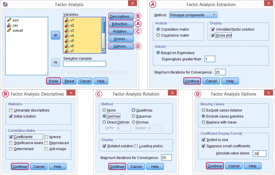
 Avoid “Exclude cases listwise” here as it'll only include our 149 “complete” respondents in our factor analysis. Clicking results in the syntax below.
SPSS Factor Analysis Syntax
set tvars both.
*Initial factor analysis as pasted from menu.
FACTOR
/VARIABLES v1 v2 v3 v4 v5 v6 v7 v8 v9 v11 v12 v13 v14 v16 v17 v20
/MISSING PAIRWISE /*IMPORTANT!*/
/PRINT INITIAL CORRELATION EXTRACTION ROTATION
/FORMAT SORT BLANK(.30)
/PLOT EIGEN
/CRITERIA MINEIGEN(1) ITERATE(25)
/EXTRACTION PC
/CRITERIA ITERATE(25)
/ROTATION VARIMAX
/METHOD=CORRELATION.
Factor Analysis Output I - Total Variance Explained
Right. Now, with 16 input variables, PCA initially extracts 16 factors (or “components”). Each component has a quality score called an Eigenvalue. Only components with high Eigenvalues are likely to represent real underlying factors.
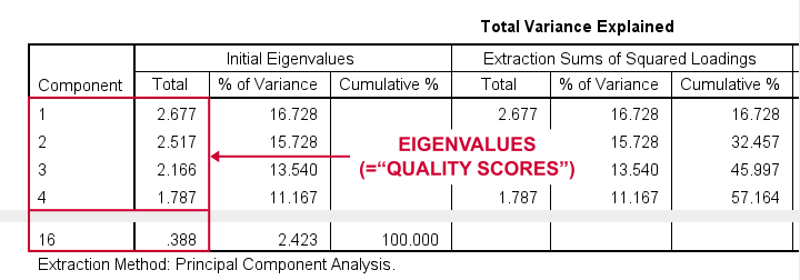
So what's a high Eigenvalue? A common rule of thumb is to select components whose Eigenvalues are at least 1. Applying this simple rule to the previous table answers our first research question: our 16 variables seem to measure 4 underlying factors.
This is because only our first 4 components have Eigenvalues of at least 1. The other components -having low quality scores- are not assumed to represent real traits underlying our 16 questions. Such components are considered “scree” as shown by the line chart below.
Factor Analysis Output II - Scree Plot
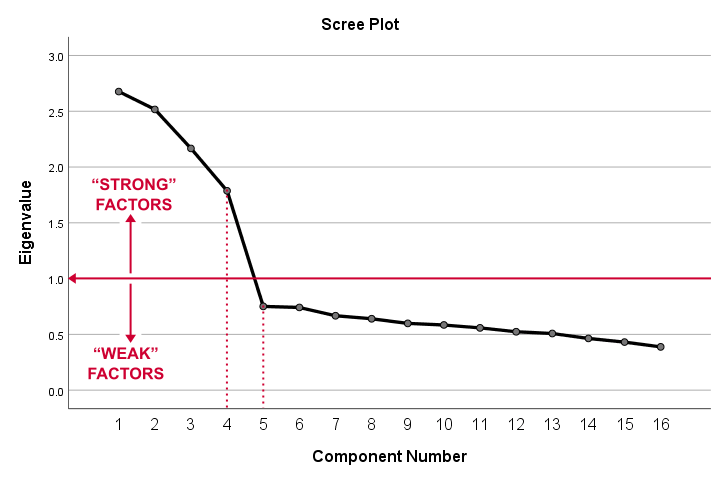
A scree plot visualizes the Eigenvalues (quality scores) we just saw. Again, we see that the first 4 components have Eigenvalues over 1. We consider these “strong factors”. After that -component 5 and onwards- the Eigenvalues drop off dramatically. The sharp drop between components 1-4 and components 5-16 strongly suggests that 4 factors underlie our questions.
Factor Analysis Output III - Communalities
So to what extent do our 4 underlying factors account for the variance of our 16 input variables? This is answered by the r square values which -for some really dumb reason- are called communalities in factor analysis.
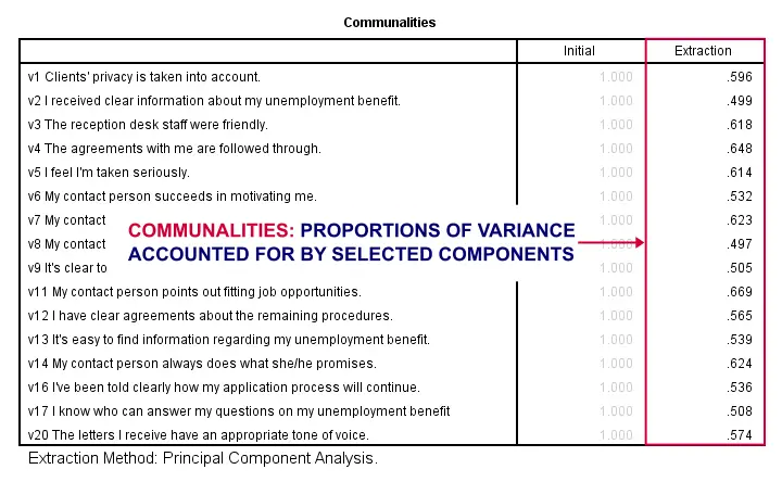
Right. So if we predict v1 from our 4 components by multiple regression, we'll find r square = 0.596 -which is v1’ s communality. Variables having low communalities -say lower than 0.40- don't contribute much to measuring the underlying factors.
You could consider removing such variables from the analysis. But keep in mind that doing so changes all results. So you'll need to rerun the entire analysis with one variable omitted. And then perhaps rerun it again with another variable left out.
If the scree plot justifies it, you could also consider selecting an additional component. But don't do this if it renders the (rotated) factor loading matrix less interpretable.
Factor Analysis Output IV - Component Matrix
Thus far, we concluded that our 16 variables probably measure 4 underlying factors. But which items measure which factors? The component matrix shows the Pearson correlations between the items and the components. For some dumb reason, these correlations are called factor loadings.
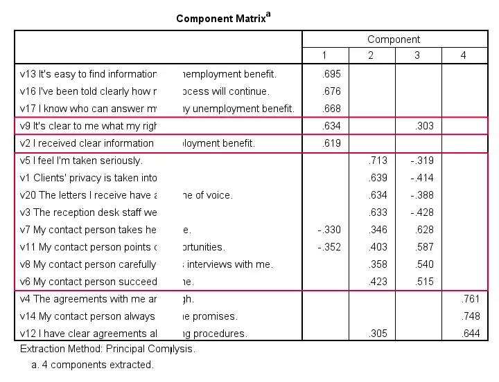
Ideally, we want each input variable to measure precisely one factor. Unfortunately, that's not the case here. For instance, v9 measures (correlates with) components 1 and 3. Worse even, v3 and v11 even measure components 1, 2 and 3 simultaneously. If a variable has more than 1 substantial factor loading, we call those cross loadings. And we don't like those. They complicate the interpretation of our factors.
The solution for this is rotation: we'll redistribute the factor loadings over the factors according to some mathematical rules that we'll leave to SPSS. This redefines what our factors represent. But that's ok. We hadn't looked into that yet anyway.
Now, there's different rotation methods but the most common one is the varimax rotation, short for “variable maximization. It tries to redistribute the factor loadings such that each variable measures precisely one factor -which is the ideal scenario for understanding our factors. And as we're about to see, our varimax rotation works perfectly for our data.
Factor Analysis Output V - Rotated Component Matrix
Our rotated component matrix (below) answers our second research question: “which variables measure which factors?”
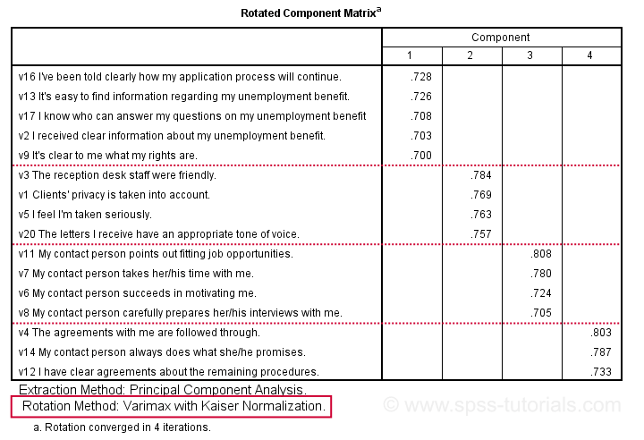
Our last research question is: “what do our factors represent?” Technically, a factor (or component) represents whatever its variables have in common. Our rotated component matrix (above) shows that our first component is measured by
- v17 - I know who can answer my questions on my unemployment benefit.
- v16 - I've been told clearly how my application process will continue.
- v13 - It's easy to find information regarding my unemployment benefit.
- v2 - I received clear information about my unemployment benefit.
- v9 - It's clear to me what my rights are.
Note that these variables all relate to the respondent receiving clear information. Therefore, we interpret component 1 as “clarity of information”. This is the underlying trait measured by v17, v16, v13, v2 and v9.
After interpreting all components in a similar fashion, we arrived at the following descriptions:
- Component 1 - “Clarity of information”
- Component 2 - “Decency and appropriateness”
- Component 3 - “Helpfulness contact person”
- Component 4 - “Reliability of agreements”
We'll set these as variable labels after actually adding the factor scores to our data.
Adding Factor Scores to Our Data
It's pretty common to add the actual factor scores to your data. They are often used as predictors in regression analysis or drivers in cluster analysis. SPSS FACTOR can add factor scores to your data but this is often a bad idea for 2 reasons:
- factor scores will only be added for cases without missing values on any of the input variables. We saw that this holds for only 149 of our 388 cases;
- factor scores are z-scores: their mean is 0 and their standard deviation is 1. This complicates their interpretation.
In many cases, a better idea is to compute factor scores as means over variables measuring similar factors. Such means tend to correlate almost perfectly with “real” factor scores but they don't suffer from the aforementioned problems. Note that you should only compute means over variables that have identical measurement scales.
It's also a good idea to inspect Cronbach’s alpha for each set of variables over which you'll compute a mean or a sum score. For our example, that would be 4 Cronbach's alphas for 4 factor scores but we'll skip that for now.
Computing and Labeling Factor Scores Syntax
compute fac_1 = mean(v16,v13,v17,v2,v9).
compute fac_2 = mean(v3,v1,v5,v20).
compute fac_3 = mean(v11,v7,v6,v8).
compute fac_4 = mean(v4,v14,v12).
*Label factors.
variable labels
fac_1 'Clarity of information'
fac_2 'Decency and appropriateness'
fac_3 'Helpfulness contact person'
fac_4 'Reliability of agreements'.
*Quick check.
descriptives fac_1 to fac_4.
Result
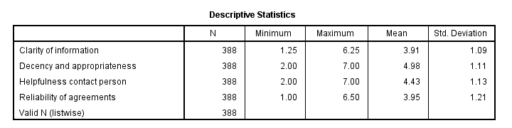
This descriptives table shows how we interpreted our factors. Because we computed them as means, they have the same 1 - 7 scales as our input variables. This allows us to conclude that
- “Decency and appropriateness” is rated best (roughly 5.0 out of 7 points) and
- “Clarity of information” is rated worst (roughly 3.9 out of 7 points).
Thanks for reading!
APA Reporting SPSS Factor Analysis
- Introduction
- Creating APA Tables - the Easy Way
- Table I - Factor Loadings & Communalities
- Table II - Total Variance Explained
- Table III - Factor Correlations
Introduction
Creating APA style tables from SPSS factor analysis output can be cumbersome. This tutorial therefore points out some tips, tricks & pitfalls. We'll use the results of SPSS Factor Analysis - Intermediate Tutorial.
All analyses are based on 20-career-ambitions-pca.sav (partly shown below).
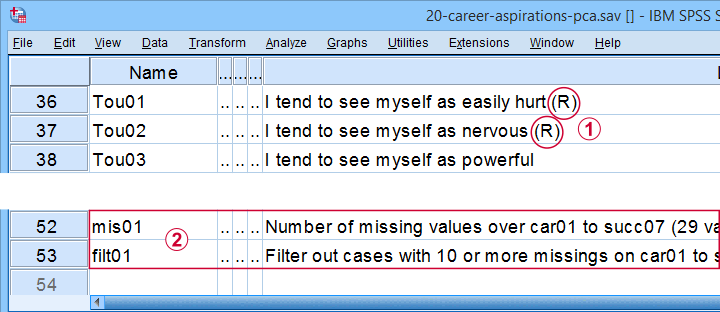
 Note that some items were reversed and therefore had “(R)” appended to their variable labels;
 We'll FILTER out cases with 10 or more missing values.
After opening these data, you can replicate the final analyses by running the SPSS syntax below.
filter by filt01.
*PCA VI - AS PREVIOUS BUT REMOVE TOU04.
FACTOR
/VARIABLES Car01 Car02 Car03 Car04 Car05 Car06 Car07 Car08 Conf01 Conf02 Conf03 Conf05 Conf06
Comp01 Comp02 Comp03 Tou01 Tou02 Tou05 Succ01 Succ02 Succ03 Succ04 Succ05 Succ06
Succ07
/MISSING PAIRWISE
/PRINT INITIAL EXTRACTION ROTATION
/FORMAT SORT BLANK(.3)
/CRITERIA FACTORS(5) ITERATE(25)
/EXTRACTION PC
/ROTATION PROMAX
/METHOD=CORRELATION.
Creating APA Tables - the Easy Way
For a wide variety of analyses, the easiest way to create APA style tables from SPSS output is usually to
- adjust your analyses in SPSS so the output is as close as possible to the desired end results. Changing table layouts (which variables/statistics go into which rows/columns?) is also best done here.
- copy-paste one or more tables into Excel or Googlesheets. This is the easiest way to set decimal places, fonts, alignment, borders and more;
- copy-paste your table(s) from Excel into WORD. Perhaps adjust the table widths with “autofit”, and you'll often have a perfect end result.
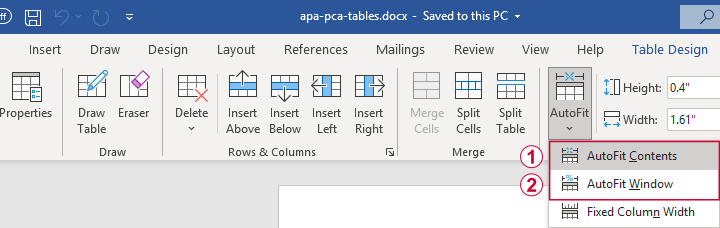 Autofit to Contents, then Window results in optimal column widths
Table I - Factor Loadings & Communalities
The figure below shows an APA style table combining factor loadings and communalities for our example analysis.
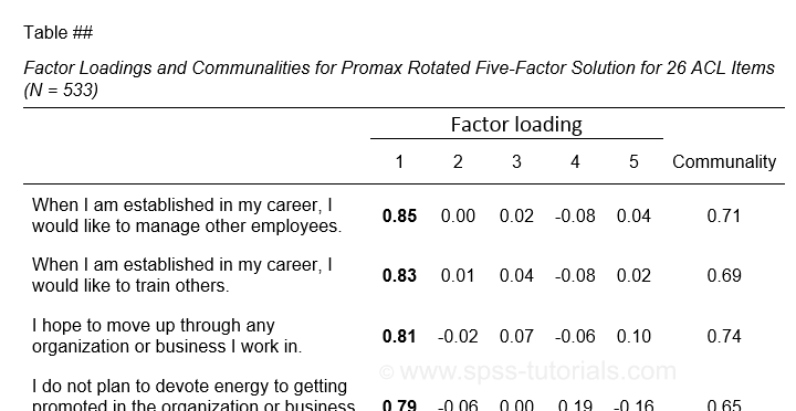 Example APA style factor loadings table
If you take a good look at the SPSS output, you'll see that you cannot simply copy-paste these tables for combining them in Excel. This is because the factor loadings (pattern matrix) table follows a different variable order than the communalities table. Since the latter follows the variable order as specified in your syntax, the easiest fix for this is to
- make sure that only variable names (not labels) are shown in the output;
- copy-paste the correctly sorted pattern matrix into Excel;
- copy-paste the variable names into the FACTOR syntax and rerun it.
Tip: try and replace the line breaks between variable names by spaces as shown below.
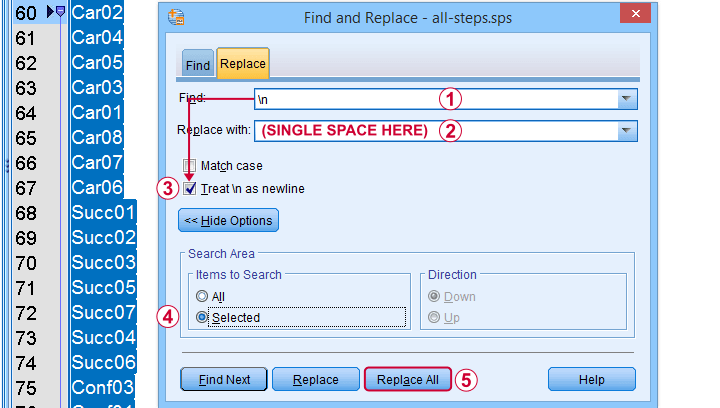 Replace line breaks by spaces in an SPSS syntax window
Also, you probably want to see only variable labels (not names) from now on. And -finally- we no longer want to hide any small absolute factor loadings shown below.
 This table is fine for an exploratory analysis but not for reporting
The syntax below does all that and thus creates output that is ideal for creating APA style tables.
set tvars labels.
*RERUN PREVIOUS ANALYSIS WITH VARIABLE ORDER AS IN PATTERN MATRIX TABLE.
FACTOR
/VARIABLES Car02 Car04 Car05 Car03 Car01 Car08 Car07 Car06 Succ01 Succ02 Succ03 Succ05 Succ07 Succ04 Succ06
Conf03 Conf01 Conf05 Conf02 Conf06 Tou02 Tou05 Tou01 Comp02 Comp03 Comp01
/MISSING PAIRWISE
/PRINT INITIAL EXTRACTION ROTATION
/FORMAT SORT
/CRITERIA FACTORS(5) ITERATE(25)
/EXTRACTION PC
/ROTATION PROMAX
/METHOD=CORRELATION.
You can now safely combine the communalities and pattern matrix tables and make some final adjustments. The end result is shown in this Googlesheet, partly shown below.
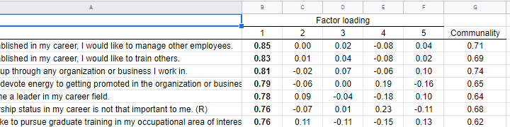 An APA table for WORD is best created in a Googlesheet or Excel
Since decimal places, fonts, alignment and borders have all been set, this table is now perfect for its final copy-paste into WORD.
Table II - Total Variance Explained
The screenshot below shows how to report the Eigenvalues table in APA style.
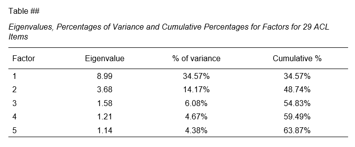 APA style Eigenvalues example table
The corresponding SPSS output table comes fairly close to this. However, an annoying problem are the missing percent signs.
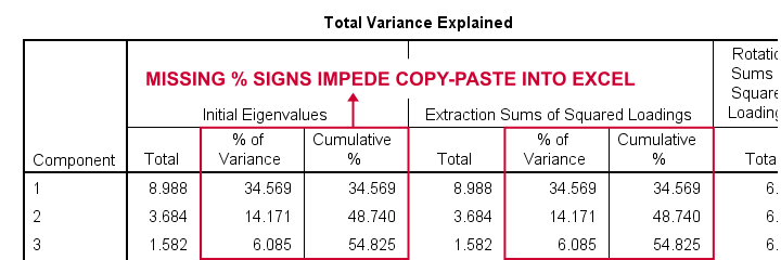
If we copy-paste into Excel and set a percentage format, 34.57 is converted into 3,457%. This is because Excel interprets these numbers as proportions rather than percentage points as SPSS does. The easiest fix is setting a percent format for these columns in SPSS before copy-pasting into Excel.
The OUTPUT MODIFY example below does just that for all Eigenvalues tables in the output window.
output modify
/select tables
/tablecells select = ["% of Variance"] format = 'pct6.2'
/tablecells select = ["Cumulative %"] format = 'pct6.2'.
After this tiny fix, you can copy-paste this table from SPSS into Excel. We can now easily make some final adjustments (including the removal of some rows and columns) and copy-paste this table into WORD.
Table III - Factor Correlations
If you used an oblique factor rotation, you'll probably want to report the correlations among your factors. The figure below shows an APA style factor correlations table.
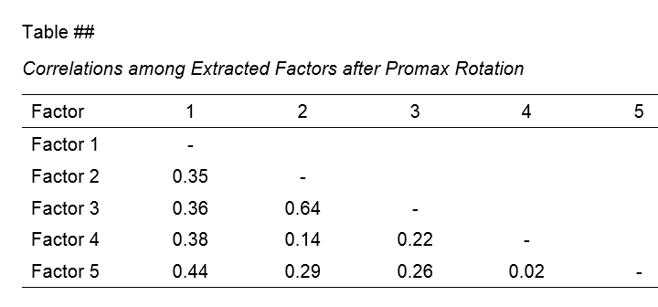
The corresponding SPSS output table (shown below) is pretty different from what we need.
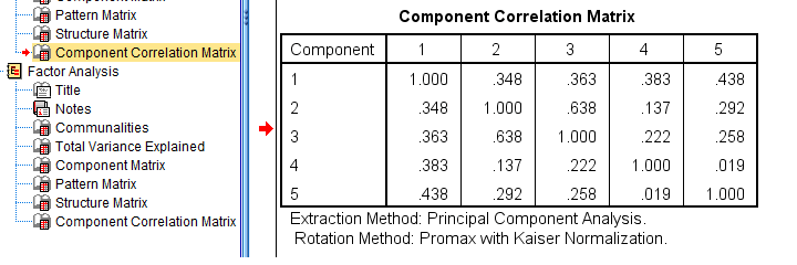 APA style factor correlation table
Adjusting this table manually is pretty doable. However, I personally prefer to use an SPSS Python script for doing so.
You can download my script from LAST-FACTOR-CORRELATION-TABLE-TO-APA.sps. This script is best run from an INSERT command as shown below.
insert file = 'D:\DOWNLOADS\LAST-FACTOR-CORRELATION-TABLE-TO-APA.sps'.
I highly recommend trying this script but it does make some assumptions:
- the above syntax assumes the script is located in D:\DOWNLOADS so you probably need to change that;
- the script assumes that you've the SPSS Python3.x essentials properly installed (usually the case for recent SPSS versions);
- the script assumes that no SPLIT FILE is in effect.
If you've any trouble or requests regarding my script, feel free to contact me and I'll see what I can do.
Final Notes
Right, so these are the basic routines I follow for creating APA style factor analysis tables. I hope you'll find them helpful.
If you've any feedback, please throw me a comment below.
Thanks for reading!
SPSS Factor Analysis – Intermediate Tutorial
- SPSS Factor Analysis Dialogs
- Output I - Total Variance Explained
- Output II - Rotated Component Matrix
- So What is a Varimax Rotation?
- Promax Rotation Reduces Cross-Loadings
- Excluding Items from Factor Analysis
Which personality traits predict career ambitions? A study was conducted to answer just that. The data -partly shown below- are in 20-career-ambitions-pca.sav.
Variables Car01 (short for “career ambitions”) through Succ07 (short for “successfulness”) attempt to measure 5 traits. These variables have already been prepared for analysis:
some negative statements were reverse coded and therefore had “(R)” appended to their variable labels;
mis01 contains the number of missing values for each respondent. We created filt01 which filters out any respondents having 10 or more missing values (out of 29 variables).
The first research questions we'd now like to answer are
- do these 29 statements indeed measure 5 underlying traits or “factors”
- precisely which statements measure which factors?
A factor analysis will answer precisely those questions. But let's first activate our filter variable by running the syntax below.
filter by filt01.
*Inspect missing values per respondent.
frequencies mis01.
Result
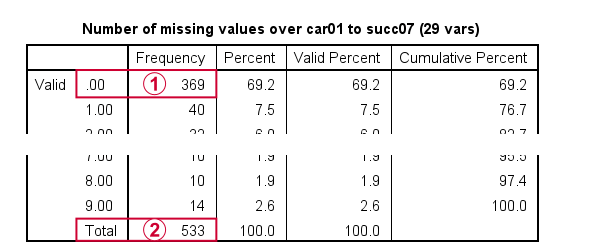
Note that only 369 out of N = 575 cases have zero missing values on all 29 variables.
With our FILTER in effect, all analyses will be limited to N = 533 cases having 9 or fewer missing values. Now, as a rule of thumb,
we'd like to use at least 15 cases for each variable
in a factor analysis.
So for our example analysis we'd like to use at least 29 (variables) * 15 = 435 cases. This is one reason for including some incomplete respondents. Another is that a larger sample size results in more statistical power and smaller confidence intervals.
Right. We're now good to go so let's proceed with our actual factor analysis.
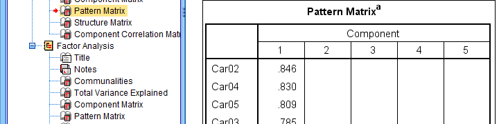
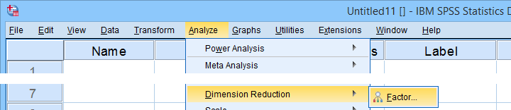
SPSS Factor Analysis Dialogs
Let's first open the factor analysis dialogs from
![]()
![]() as shown below.
as shown below.
For our first analysis, most default settings will do. However, we do want to adjust some settings under Rotation and Options.
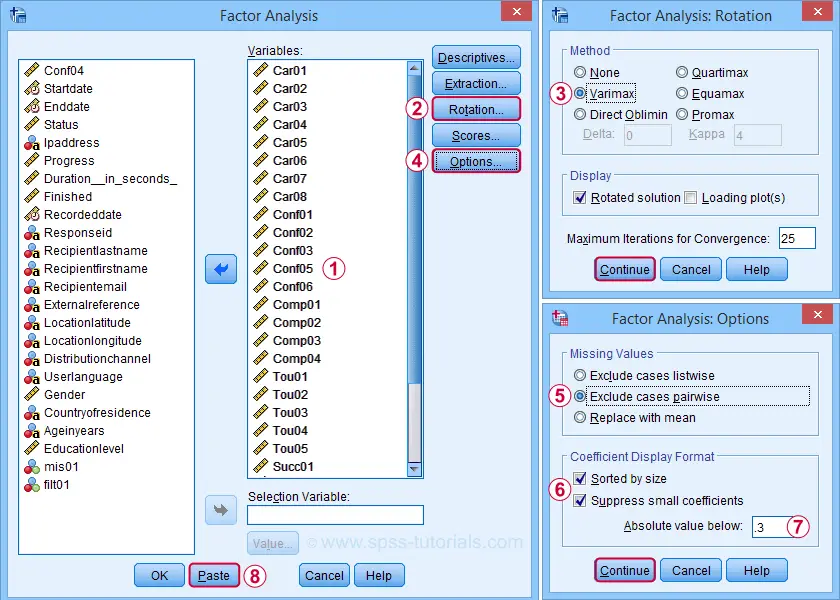
 We'll exclude cases with missing values pairwise. Listwise exclusion limits our analysis to N = 369 complete cases which is (arguably) insufficient sample size for 29 variables.
Completing these steps results in the syntax below.
SPSS FACTOR Syntax I - Basic Settings
FACTOR
/VARIABLES Car01 Car02 Car03 Car04 Car05 Car06 Car07 Car08 Conf01 Conf02 Conf03 Conf05 Conf06
Comp01 Comp02 Comp03 Comp04 Tou01 Tou02 Tou03 Tou04 Tou05 Succ01 Succ02 Succ03 Succ04 Succ05 Succ06
Succ07
/MISSING PAIRWISE
/ANALYSIS Car01 Car02 Car03 Car04 Car05 Car06 Car07 Car08 Conf01 Conf02 Conf03 Conf05 Conf06
Comp01 Comp02 Comp03 Comp04 Tou01 Tou02 Tou03 Tou04 Tou05 Succ01 Succ02 Succ03 Succ04 Succ05 Succ06
Succ07
/PRINT INITIAL EXTRACTION ROTATION
/FORMAT SORT BLANK(.3)
/CRITERIA MINEIGEN(1) ITERATE(25)
/EXTRACTION PC
/CRITERIA ITERATE(25)
/ROTATION VARIMAX
/METHOD=CORRELATION.
In this syntax, the ANALYSIS and second CRITERIA subcommands are redundant. Removing them keeps the syntax tidy and makes it easier to copy-paste-edit it for subsequent analyses. I therefore prefer to use the shortened syntax below.
FACTOR
/VARIABLES Car01 Car02 Car03 Car04 Car05 Car06 Car07 Car08 Conf01 Conf02 Conf03 Conf05 Conf06
Comp01 Comp02 Comp03 Comp04 Tou01 Tou02 Tou03 Tou04 Tou05 Succ01 Succ02 Succ03 Succ04 Succ05 Succ06
Succ07
/MISSING PAIRWISE
/PRINT INITIAL EXTRACTION ROTATION
/FORMAT SORT BLANK(.3)
/CRITERIA MINEIGEN(1) ITERATE(25)
/EXTRACTION PC
/ROTATION VARIMAX
/METHOD=CORRELATION.
SPSS FACTOR Output I - Total Variance Explained
After running our first factor analysis, let's first inspect the Total Variance Explained Table (shown below).
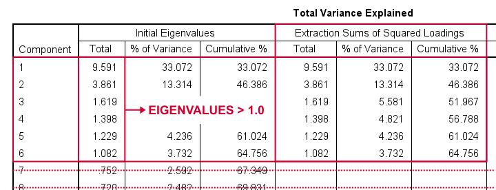
This table tells us that
- SPSS has created 29 artificial variables known as components.
- These components aim to represent personality traits underlying our analysis variables (“items”).
- If a component reflects a real trait, it should correlate substantially with these items. Or put differently: it should account for a reasonable percentage of variance.
- Like so, component 1 accounts for 33.07% of the variance in our 29 items or an equivalent of 9.59 items. This number is known as an eigenvalue.
- You could thus think of eigenvalues as “quality scores” for the components: higher eigenvalues provide stronger evidence that components represent real underlying traits. Now, the big question is:
which components have sufficient eigenvalues
to be considered real traits?
By default, SPSS uses a cutoff value of 1.0 for eigenvalues. This is because the average eigenvalue is always 1.0 if you analyze correlations. Therefore, this rule of thumb is completely arbitrary: there's no real reason why 1.0 should be better cutoff value than 0.8 or 1.2.
In any case, SPSS suggests that our 29 items may measure 6 underlying traits. We'd now like to know which items measure which traits. For answering this, we inspect the Rotated Component Matrix shown below.
SPSS FACTOR Output II - Rotated Component Matrix
The Rotated Component Matrix contains the Pearson correlations between items and components or “factors”. These are known as factor loadings and allow us to interpret which traits our components may reflect.
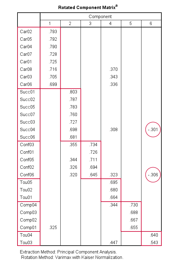
- Component 1 correlates strongly with Car02, Car05,..., Car06. If we inspect the variable labels of these variables, we see that the “Car” items all relate to career ambitions. Therefore, component 1 seems to reflect some kind of career ambition trait.
- Component 2 correlates mostly with the “Succ” items. Their variable labels tell us that these items relate to successfulness.
- In a similar vein, Component 3 correlates most with the self confidence items Conf01 to Conf05.
- Component 4 seems to measure toughness.
- Component 5 may reflect a competitiveness trait.
- Component 6 correlates somewhat positively with 2 toughness items but somewhat negatively with a successfulness and confidence item. As none of these loadings are very strong, component 6 is not easily interpretable.
These results suggest that perhaps only components 1-5 reflect real underlying traits. Now, the table we just inspected shows the factor loadings after a varimax rotation of our 6 components (or “factors”).
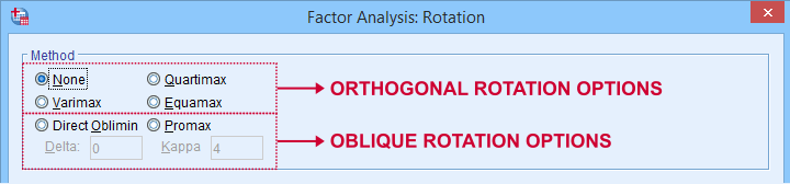
So What is a Varimax Rotation?
Very basically,
a factor rotation is a mathematical procedure that
redistributes factor loadings over factors.
The reason for doing this is that this makes our factors easier to interpret: rotation typically causes each item to load highly on precisely one factor. There's different factor rotation methods but all of them fall into 2 basic types:
- an orthogonal rotation does not allow any factors to correlate with each other. An example is the varimax rotation.
- an oblique rotation allows all factors to correlate with each other. Examples are the promax and oblimin rotations.
Now, factor rotation also redistributes the percentages of variance accounted for by different factors. The new percentages are shown below under Rotation Sums of Squared Loadings.
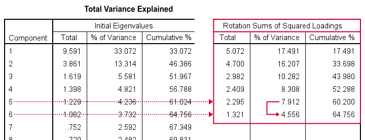
What's striking here, is the huge drop from component 5 (7.91%) to component 6 (4.56%). This provides further evidence that our items perhaps measure 5 rather than 6 underlying factors.
We'll therefore rerun our analysis and force SPSS to extract and rotate 5 instead of 6 factors. We'll do so by copy-pasting our first syntax and replacing MINEIGEN(1) by FACTORS(5).
SPSS FACTOR Syntax II - Force 5 Factor Solution
FACTOR
/VARIABLES Car01 Car02 Car03 Car04 Car05 Car06 Car07 Car08 Conf01 Conf02 Conf03 Conf05 Conf06
Comp01 Comp02 Comp03 Comp04 Tou01 Tou02 Tou03 Tou04 Tou05 Succ01 Succ02 Succ03 Succ04 Succ05 Succ06
Succ07
/MISSING PAIRWISE
/PRINT INITIAL EXTRACTION ROTATION
/FORMAT SORT BLANK(.3)
/CRITERIA FACTORS(5) ITERATE(25)
/EXTRACTION PC
/ROTATION VARIMAX
/METHOD=CORRELATION.
Result
Our rotated component matrix looks much better now: each component is interpretable and has some strong positive factor loadings. The negative loadings are all gone.
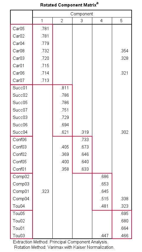
Promax Rotation Reduces Cross-Loadings
A problem with this solution, though, is that many items load on 2 or more factors simultaneously. Such secondary loadings are known as cross-loadings and conflict with the basic factor model as shown below.
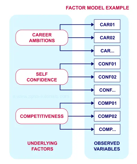
Each item measures only one trait and should thus load substantially on only one factor. Also note that there's no arrows among the underlying factors: the model claims that
career ambitions, self confidence and competitiveness
are all perfectly uncorrelated.
Does anybody think that's realistic for real-world data? I sure don't. Of course such traits are correlated substantially. However, our varimax rotation does not allow our factors to correlate. And therefore, these correlations express themselves as cross-loadings.
With most data, cross-loadings disappear when we allow our factors to correlate. We'll do just that by using an oblique factor rotation such as promax.
SPSS FACTOR Syntax III - Promax Rotation
FACTOR
/VARIABLES Car01 Car02 Car03 Car04 Car05 Car06 Car07 Car08 Conf01 Conf02 Conf03 Conf05 Conf06
Comp01 Comp02 Comp03 Comp04 Tou01 Tou02 Tou03 Tou04 Tou05 Succ01 Succ02 Succ03 Succ04 Succ05 Succ06
Succ07
/MISSING PAIRWISE
/PRINT INITIAL EXTRACTION ROTATION
/FORMAT SORT BLANK(.3)
/CRITERIA FACTORS(5) ITERATE(25)
/EXTRACTION PC
/ROTATION PROMAX
/METHOD=CORRELATION.
Result
When using an oblique rotation, we usually inspect the Pattern Matrix for interpreting our components.
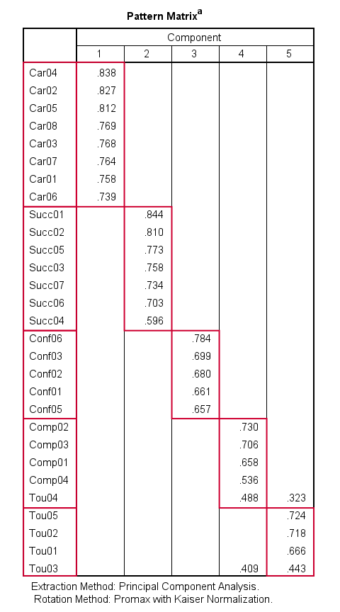
Our pattern matrix looks great! Almost all cross-loadings have gone. But where did they go? Well, correlations among factors have taken over their role. This typically happens during an oblique rotation. These correlations are shown in the Component Correlation Matrix, the last table in our output.
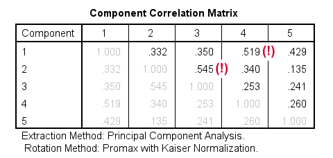
Most correlations indicate medium or even strong effect sizes. I think that's perfectly realistic: our components reflect traits such as successfulness and self confidence and these are obviously strongly correlated in the real world.
Personally, I'd settle for the variable grouping proposed by this analysis. A good next step is inspecting Cronbach’s alphas for our 5 subscales. Finally, we'd create subscale scores in our data by computing means over these variables and perhaps proceed with a regression analysis.
Excluding Items from Factor Analysis
Most textbooks propose that you now exclude items with cross-loadings from the analysis. For our analysis, SPSS shows absolute loadings < 0.3 as blanks. This cutoff value -although completely arbitrary- seems a reasonable threshold for separating negligible from substantial loadings.
Anyway, if you decide to exclude items, the right way to do so is to
- look up the variable having the highest cross-loading;
- remove its variable name from the FACTOR syntax;
- rerun the factor analysis -note that all loadings now change;
- repeat these steps if necessary and keep track of what you're doing.
For our example analysis, these steps result in the syntax below.
FACTOR
/VARIABLES Car01 Car02 Car03 Car04 Car05 Car06 Car07 Car08 Conf01 Conf02 Conf03 Conf05 Conf06
Comp01 Comp02 Comp03 Comp04 Tou01 Tou02 Tou04 Tou05 Succ01 Succ02 Succ03 Succ04 Succ05 Succ06
Succ07
/MISSING PAIRWISE
/PRINT INITIAL EXTRACTION ROTATION
/FORMAT SORT BLANK(.3)
/CRITERIA FACTORS(5) ITERATE(25)
/EXTRACTION PC
/ROTATION PROMAX
/METHOD=CORRELATION.
*PCA V - AS PREVIOUS BUT REMOVE COMP04.
FACTOR
/VARIABLES Car01 Car02 Car03 Car04 Car05 Car06 Car07 Car08 Conf01 Conf02 Conf03 Conf05 Conf06
Comp01 Comp02 Comp03 Tou01 Tou02 Tou04 Tou05 Succ01 Succ02 Succ03 Succ04 Succ05 Succ06
Succ07
/MISSING PAIRWISE
/PRINT INITIAL EXTRACTION ROTATION
/FORMAT SORT BLANK(.3)
/CRITERIA FACTORS(5) ITERATE(25)
/EXTRACTION PC
/ROTATION PROMAX
/METHOD=CORRELATION.
*PCA VI - AS PREVIOUS BUT REMOVE TOU04.
FACTOR
/VARIABLES Car01 Car02 Car03 Car04 Car05 Car06 Car07 Car08 Conf01 Conf02 Conf03 Conf05 Conf06
Comp01 Comp02 Comp03 Tou01 Tou02 Tou05 Succ01 Succ02 Succ03 Succ04 Succ05 Succ06
Succ07
/MISSING PAIRWISE
/PRINT INITIAL EXTRACTION ROTATION
/FORMAT SORT BLANK(.3)
/CRITERIA FACTORS(5) ITERATE(25)
/EXTRACTION PC
/ROTATION PROMAX
/METHOD=CORRELATION.
Result
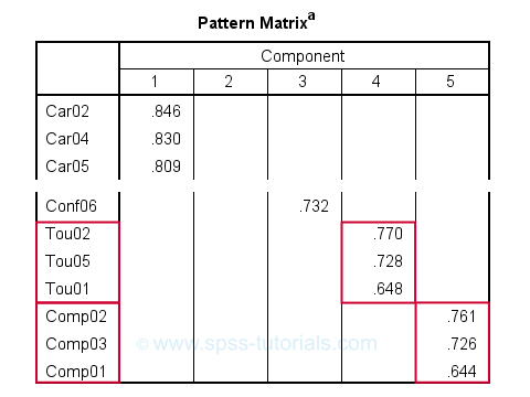
After removing 3 items with cross-loadings, it seems we've a perfectly clean factor structure: each item seems to load on precisely one factor. Keep in mind, however, that we chose to suppress absolute loadings < 0.30. Those are not shown but they still exist.
Right, I guess that'll do for today. I hope you found this tutorial helpful. And last but not least,
Thanks for reading!