Chi-Square Goodness-of-Fit Test – Simple Tutorial

• Null Hypothesis
• Assumptions
• Formulas
• Effect Size - Cohen’s W
• Power and Sample Size Calculation

A chi-square goodness-of-fit test examines if a categorical variable
has some hypothesized frequency distribution in some population. The chi-square goodness-of-fit test is also known as

• one-sample chi-square test (SPSS) or
• multinomial test (JASP).

Example - Testing Car Advertisements

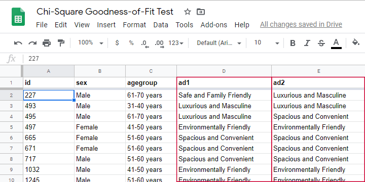
A car manufacturer wants to launch a campaign for a new car. They'll show advertisements -or “ads”- in 4 different sizes. For ad each size, they have 4 ads that try to convey some message such as “this car is environmentally friendly”. They then asked N = 80 people which ad they liked most. The data thus obtained are in this Googlesheet, partly shown below.

So which ads performed best in our sample? Well, we can simply look up which ad was preferred by most respondents: the ad having the highest frequency is the mode for each ad size.

So let's have a look at the frequency distribution for the first ad size -ad1- as visualized in the bar chart shown below.

Observed Frequencies and Bar Chart

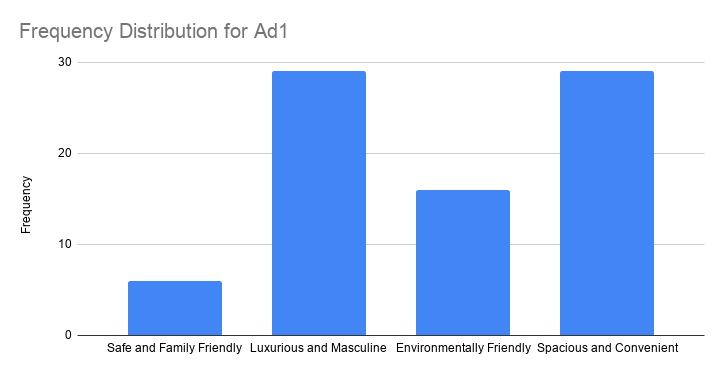
The observed frequencies shown in this chart are

1. Safe and Family Friendly: 6
2. Luxurious and Masculine: 29
3. Environmentally Friendly: 16
4. Spacious and Convenient: 29

Note that ad1 has a bimodal distribution: ads 2 and 4 are both winners with 29 votes. However, our data only hold a sample of N = 80. So can we conclude that ads 2 and 4
also perform best in the entire population? The chi-square goodness-of-fit answers just that. And for this example, it does so by trying to reject the null hypothesis that all ads perform equally well in the population.

Null Hypothesis

Generally, the null hypothesis for a chi-square goodness-of-fit test is simply

$$H_0: P_{01}, P_{02},...,P_{0m},\; \sum_{i=0}^m\biggl(P_{0i}\biggr) = 1$$

where \(P_{0i}\) denote population proportions for \(m\) categories in some categorical variable. You can choose any set of proportions as long as they add up to one. In many cases, all proportions being equal is the most likely null hypothesis.
For a dichotomous variable having only 2 categories, you're better off using

• a binomial test because it gives the exact instead of the approximate significance level or
• a z-test for 1 proportion because it gives a confidence interval for the population proportion.

Anyway, for our example, we'd like to show that some ads perform better than others. So we'll try to refute that our 4 population proportions are all equal and -hence- 0.25.

Expected Frequencies

Now, if the 4 population proportions really are 0.25 and we sample N = 80 respondents, then we expect each ad to be preferred by 0.25 · 80 = 20 respondents. That is, all 4 expected frequencies are 20. We need to know these expected frequencies for 2 reasons:

• computing our test statistic requires expected frequencies and
• the assumptions for the chi-square goodness-of-fit test involve expected frequencies as well.

Assumptions

The chi-square goodness-of-fit test requires 2 assumptions^2,3:

1. independent observations;
2. for 2 categories, each expected frequency \(Ei\) must be at least 5.
   For 3+ categories, each \(Ei\) must be at least 1 and no more than 20% of all \(Ei\) may be smaller than 5.

The observations in our data are independent because they are distinct persons who didn't interact while completing our survey. We also saw that all \(Ei\) are (0.25 · 80 =) 20 for our example. So this second assumption is met as well.

Formulas

We'll first compute the \(\chi^2\) test statistic as

$$\chi^2 = \sum\frac{(O_i - E_i)^2}{E_i}$$

where

• \(O_i\) denotes the observed frequencies and
• \(E_i\) denotes the expected frequencies -usually all equal.

For ad1, this results in

$$\chi^2 = \frac{(16 - 20)^2}{20} + \frac{(29 - 20)^2}{20} + \frac{(9 - 20)^2}{20} + \frac{(29 - 20)^2}{20} = 18.7 $$

If all assumptions have been met, \(\chi^2\) approximately follows a chi-square distribution with \(df\) degrees of freedom where

$$df = m - 1$$

for \(m\) frequencies. Since we have 4 frequencies for 4 different ads,

$$df = 4 - 1 = 3$$

for our example data. Finally, we can simply look up the significance level as

$$P(\chi^2(3) > 18.7) \approx 0.00032$$

We ran these calculations in this Googlesheet shown below.

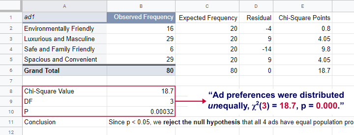
So what does this mean? Well, if all 4 ads are equally preferred in the population, there's a 0.00032 chance of finding our observed frequencies. Since p < 0.05, we reject the null hypothesis. Conclusion: some ads are preferred by more people than others in the entire population of readers.

Right, so it's safe to assume that the population proportions are not all equal. But precisely how different are they? We can express this in a single number: the effect size.

Effect Size - Cohen’s W

The effect size for a chi-square goodness-of-fit test -as well as the chi-square independence test- is Cohen’s W. Some rules of thumb¹ are that

• Cohen’s W = 0.10 indicates a small effect size;
• Cohen’s W = 0.30 indicates a medium effect size;
• Cohen’s W = 0.50 indicates a large effect size.

Cohen’s W is computed as

$$W = \sqrt{\sum_{i = 1}^m\frac{(P_{oi} - P_{ei})^2}{P_{ei}}}$$

where

• \(P_{oi}\) denote observed proportions and
• \(P_{ei}\) denote expected proportions under the null hypothesis for
• \(m\) cells.

For ad1, the null hypothesis states that all expected proportions are 0.25. The observed proportions are computed from the observed frequencies (see screenshot below) and result in

$$W = \sqrt{\frac{(0.2 - 0.25)^2}{0.25} +\frac{(0.3625 - 0.25)^2}{0.25} +\frac{(0.075 - 0.25)^2}{0.25} +\frac{(0.3625 - 0.25)^2}{0.25} } = $$

$$W = \sqrt{0.234} = 0.483$$

We ran these computations in this Googlesheet shown below.

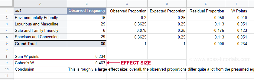
For ad1, the effect size \(W\) = 0.483. This indicates a large overall difference between the observed and expected frequencies.

Power and Sample Size Calculation

Now that we computed our effect size, we're ready for our last 2 steps. First off, what about power? What's the probability demonstrating an effect if

• we test at α = 0.05;
• we have a sample of N = 80;
• df = 3 (our outcome variable has 4 categories);
• we don't know the population effect size \(W\)?

The chart below -created in G*Power- answers just that.

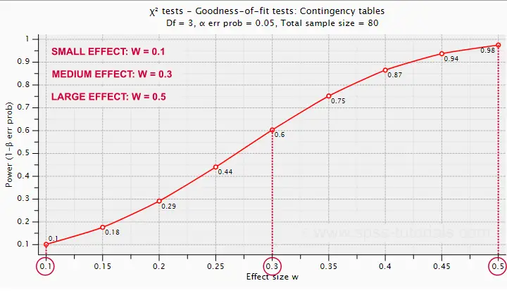
Some basic conclusions are that

• power = 0.98 for a large effect size;
• power = 0.60 for a medium effect size;
• power = 0.10 for a small effect size.

These outcomes are not too great: we only have a 0.60 probability of rejecting the null hypothesis if the population effect size is medium and N = 80. However, we can increase power by increasing the sample size. So which sample sizes do we need if

• we test at α = 0.05;
• we want to have power = 0.80;
• df = 3 (our outcome variable has 4 categories);
• we don't know the population effect size \(W\)?

The chart below shows how required sample sizes decrease with increasing effect sizes.

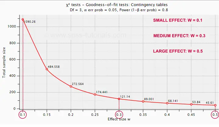
Under the aforementioned conditions, we have power ≥ 0.80

• for a large effect size if N = 44;
• for a medium effect size if N = 122;
• for a small effect size if N = 1091.

References

1. Cohen, J (1988). Statistical Power Analysis for the Social Sciences (2nd. Edition). Hillsdale, New Jersey, Lawrence Erlbaum Associates.
2. Siegel, S. & Castellan, N.J. (1989). Nonparametric Statistics for the Behavioral Sciences (2nd ed.). Singapore: McGraw-Hill.
3. Warner, R.M. (2013). Applied Statistics (2nd. Edition). Thousand Oaks, CA: SAGE.

SPSS One Sample Chi-Square Test

SPSS one-sample chi-square test is used to test whether a single categorical variable follows a hypothesized population distribution.

SPSS One-Sample Chi-Square Test Example

A marketeer believes that 4 smartphone brands are equally attractive. He asks 43 people which brand they prefer, resulting in brands.sav. If the brands are really equally attractive, each brand should be chosen by roughly the same number of respondents. In other words, the expected frequencies under the null hypothesis are (43 cases / 4 brands =) 10.75 cases for each brand. The more the observed frequencies differ from these expected frequencies, the less likely it is that the brands really are equally attractive.

1. Quick Data Check

Before running any statistical tests, we always want to have an idea what our data basically look like. In this case we'll inspect a histogram of the preferred brand by running FREQUENCIES. We'll open the data file and create our histogram by running the syntax below. Since it's very simple, we won't bother about clicking through the menu here.

First, N = 43 means that the histogram is based on 43 cases. Since this is our sample size, we conclude that no missing values are present. SPSS also calculates a mean and standard deviation but these are not meaningful for nominal variables so we'll just ignore them. Second, the preferred brands have rather unequal frequencies, casting some doubt upon the null hypothesis of those being equal in the population.

Assumptions One-Sample Chi-Square Test

1. independent and identically distributed variables (or “independent observations”);
2. none of the expected frequencies are < 5;

The first assumption is beyond the scope of this tutorial. We'll presume it's been met by our data. Whether the assumption 2 holds is reported by SPSS whenever we run a one-sample chi-square test. However, we already saw that all expected frequencies are 10.75 for our data.

3. Run SPSS One Sample Chi-Square Test

Expected Values refers to the expected frequencies, the aforementioned 10.75 cases for each brand. We could enter these values but selecting All categories equal is a faster option and yields identical results.
Clicking Paste results in the syntax below.

4. SPSS One-Sample Chi-Square Test Output

Under Observed N we find the observed frequencies that we saw previously;
under Expected N we find the theoretically expected frequencies;They're shown as 10.8 instead of 10.75 due to rounding. All reported decimals can be seen by double-clicking the value.
for each frequency the Residual is the difference between the observed and the expected frequency and thus expresses a deviation from the null hypothesis;
the Chi-Square test statistic sort of summarizes the residuals and hence indicates the overall difference between the data and the hypothesis. The larger the chi-square value, the less the data “fit” the null hypothesis;
degrees of freedom (df) specifies which chi-square distribution applies;
Asymp. Sig. refers to the p value and is .073 in this case. If the brands are exactly equally attractive in the population, there's a 7.3% chance of finding our observed frequencies or a larger deviation from the null hypothesis. We usually reject the null hypothesis if p < .05. Since this is not the case, we conclude that the brands are equally attractive in the population.

Reporting a One-Sample Chi-Square Test

When reporting a one-sample chi-square test, we always report the observed frequencies. The expected frequencies usually follow readily from the null hypothesis so reporting them is optional. Regarding the significance test, we usually write something like “we could not demonstrate that the four brands are not equally attractive; χ²(3) = 6.95, p = .073.”