- ANCOVA - Null Hypothesis
- ANCOVA Assumptions
- SPSS ANCOVA Dialogs
- SPSS ANCOVA Output - Between-Subjects Effects
- SPSS ANCOVA Output - Adjusted Means
- ANCOVA - APA Style Reporting
A pharmaceutical company develops a new medicine against high blood pressure. They tested their medicine against an old medicine, a placebo and a control group. The data -partly shown below- are in blood-pressure.sav.
Our company wants to know if their medicine outperforms the other treatments: do these participants have lower blood pressures than the others after taking the new medicine? Since treatment is a nominal variable, this could be answered with a simple ANOVA.
Now, posttreatment blood pressure is known to correlate strongly with pretreatment blood pressure. This variable should therefore be taken into account as well. The relation between pretreatment and posttreatment blood pressure could be examined with simple linear regression because both variables are quantitative.
We'd now like to examine the effect of medicine while controlling for pretreatment blood pressure. We can do so by adding our pretest as a covariate to our ANOVA. This now becomes ANCOVA -short for analysis of covariance. This analysis basically combines ANOVA with regression.
Surprisingly, analysis of covariance does not actually involve covariances as discussed in Covariance - Quick Introduction.
ANCOVA - Null Hypothesis
Generally, ANCOVA tries to demonstrate some effect by rejecting the null hypothesis that all population means are equal when controlling for 1+ covariates. For our example, this translates to “average posttreatment blood pressures are equal for all treatments when controlling for pretreatment blood pressure”. The basic analysis is pretty straightforward but it does require quite a few assumptions. Let's look into those first.
ANCOVA Assumptions
- independent observations;
- normality: the dependent variable must be normally distributed within each subpopulation. This is only needed for small samples of n < 20 or so;
- homogeneity: the variance of the dependent variable must be equal over all subpopulations. This is only needed for sharply unequal sample sizes;
- homogeneity of regression slopes: the b-coefficient(s) for the covariate(s) must be equal among all subpopulations.
- linearity: the relation between the covariate(s) and the dependent variable must be linear.
Taking these into account, a good strategy for our entire analysis is to
- first run some basic data checks: histograms and descriptive statistics give quick insights into frequency distributions and sample sizes. This tells us if we even need assumptions 2 and 3 in the first place.
- see if assumptions 4 and 5 hold by running regression analyses for our treatment groups separately;
- run the actual ANCOVA and see if assumption 3 -if necessary- holds.
Data Checks I - Histograms
Let's first see if our blood pressure variables are even plausible in the first place. We'll inspect their histograms by running the syntax below. If you prefer to use SPSS’ menu, consult Creating Histograms in SPSS.
frequencies predias postdias
/format notable
/histogram.
Result
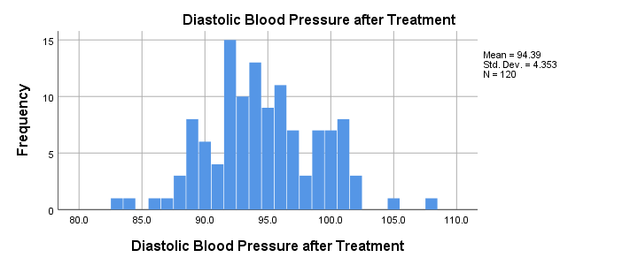
Conclusion: the frequency distributions for our blood pressure measurements look plausible: we don't see any very low or high values. Neither shows a lot of skewness or kurtosis and they both look reasonably normally distributed.
Data Checks II - Descriptive Statistics
Next, let's look into some descriptive statistics, especially sample sizes. We'll create and inspect a table with the
- sample sizes,
- means and
- standard deviations
of the outcome variable and the covariate for our treatment groups separately. We could do so from
![]()
![]() or -faster- straight from syntax.
or -faster- straight from syntax.
means predias postdias by treatment
/statistics anova.
Result
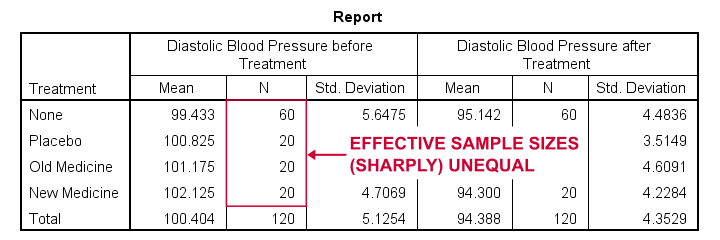
The main conclusions from our output are that
- all treatment groups have reasonable samples sizes of at least n = 20. This means we don't need to bother about the normality assumption. Otherwise, we could use a Shapiro-Wilk normality test or a Kolmogorov-Smirnov test but we rather avoid these.
- the treatment groups have sharply unequal sample sizes. This implies that our ANCOVA will need to satisfy the homogeneity of variance assumption.
- the ANOVA results (not shown here) tell us that the posttreatment means don't differ statistically significantly, F(3,116) = 1.619, p = 0.189. However, this test did not yet include our covariate -pretreatment blood pressure.
So much for our basic data checks. We'll now look into the regression results and then move on to the actual ANCOVA.
Separate Regression Lines for Treatment Groups
Let's now see if our regression slopes are equal among groups -one of the ANCOVA assumptions. We'll first just visualize them in a scatterplot as shown below.
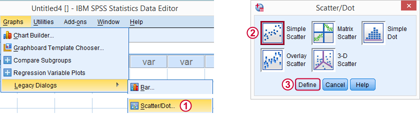
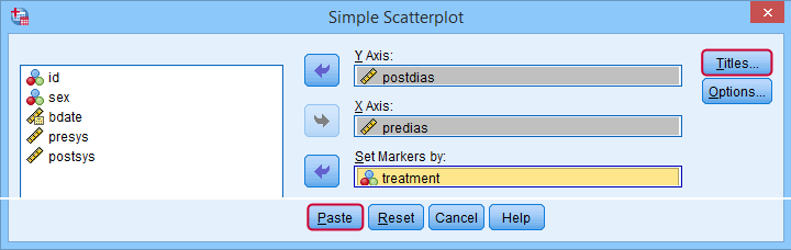
Clicking results in the syntax below.
GRAPH
/SCATTERPLOT(BIVAR)=predias WITH postdias BY treatment
/MISSING=LISTWISE.GRAPH
/TITLE='Diastolic Blood Pressure by Treatment'.
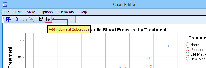
*Double-click resulting chart and click "Add fit line at subgroups" icon.
SPSS now creates a scatterplot with different colors for different treatment groups. Double-clicking it opens it in a Chart Editor window. Here we click the “Add Fit Lines at Subgroups” icon as shown below.
Result
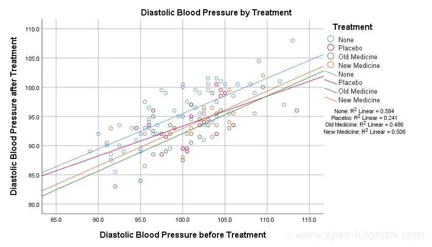
The main conclusion from this chart is that the regression lines are almost perfectly parallel: our data seem to meet the homogeneity of regression slopes assumption required by ANCOVA.
Furthermore, we don't see any deviations from linearity: this ANCOVA assumption also seems to be met. For a more thorough linearity check, we could run the actual regressions with residual plots. We did just that in SPSS Moderation Regression Tutorial.
Now that we checked some assumptions, we'll run the actual ANCOVA twice:
- the first run only examines the homogeneity of regression slopes assumption. If this holds, then there should not be any covariate by treatment interaction-effect.
- the second run tests our null hypothesis: are all population means equal when controlling for our covariate?
SPSS ANCOVA Dialogs
Let's first navigate to
![]()
![]() and fill out the dialog boxes as shown below.
and fill out the dialog boxes as shown below.
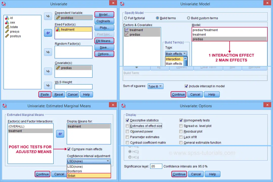
Clicking generates the syntax shown below.
UNIANOVA postdias BY treatment WITH predias
/METHOD=SSTYPE(3)
/INTERCEPT=INCLUDE
/EMMEANS=TABLES(treatment) WITH(predias=MEAN) COMPARE ADJ(SIDAK)
/PRINT ETASQ HOMOGENEITY
/CRITERIA=ALPHA(.05)
/DESIGN=predias treatment predias*treatment. /* predias*treatment adds interaction effect to model.
Result
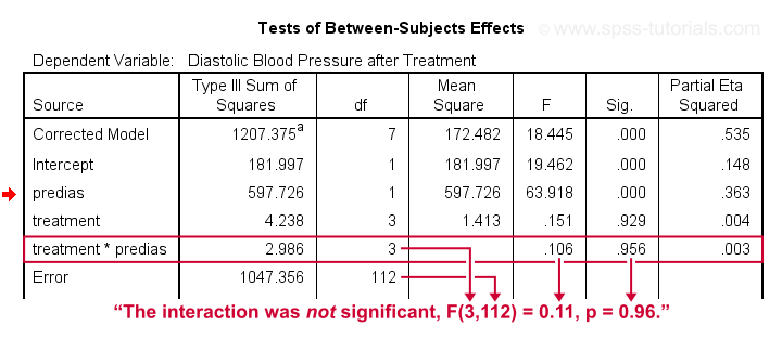
First note that our covariate by treatment interaction is not statistically significant at all: F(3,112) = 0.11, p = 0.96. This means that the regression slopes for the covariate don't differ between treatments: the homogeneity of regression slopes assumption seems to hold almost perfectly.
For these data, this doesn't come as a surprise: we already saw that the regression lines for different treatment groups were roughly parallel. Our first ANCOVA is basically a more formal way to make the same point.
SPSS ANCOVA II - Main Effects
We now run simply rerun our ANCOVA as previously. This time, however, we'll remove the covariate by treatment interaction effect. Doing so results in the syntax shown below.
UNIANOVA postdias BY treatment WITH predias
/METHOD=SSTYPE(3)
/INTERCEPT=INCLUDE
/EMMEANS=TABLES(treatment) WITH(predias=MEAN) COMPARE ADJ(SIDAK)
/PRINT ETASQ HOMOGENEITY
/CRITERIA=ALPHA(.05)
/DESIGN=predias treatment. /* only test for 2 main effects.
SPSS ANCOVA Output I - Levene's Test
Since our treatment groups have sharply unequal sample sizes, our data need to satisfy the homogeneity of variance assumption. This is why we included Levene's test in our analysis. Its results are shown below.
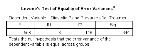
Conclusion: we don't reject the null hypothesis of equal error variances, F(3,116) = 0.56, p = 0.64. Our data meets the homogeneity of variances assumption. This means we can confidently report the other results.
SPSS ANCOVA Output - Between-Subjects Effects
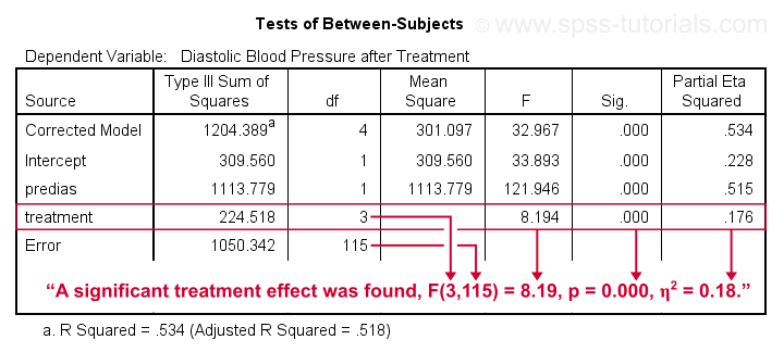
Conclusion: we reject the null hypothesis that our treatments result in equal mean blood pressures, F(3,115) = 8.19, p = 0.000.
Importantly, the effect size for treatment is between medium and large: partial eta squared (written as η2) = 0.176.
Apparently, some treatments perform better than others after all. Interestingly, this treatment effect was not statistically significant before including our pretest as a covariate.
So which treatments perform better or worse? For answering this, we first inspect our estimated marginal means table.
SPSS ANCOVA Output - Adjusted Means
One role of covariates is to adjust posttest means for any differences among the corresponding pretest means. These adjusted means and their standard errors are found in the Estimated Marginal Means table shown below.
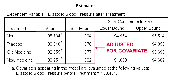
These adjusted means suggest that all treatments result in lower mean blood pressures than “None”. The lowest mean blood pressure is observed for the old medicine. So precisely which mean differences are statistically significant? This is answered by post hoc tests which are found in the Pairwise Comparisons table (not shown here). This table shows that all 3 treatments differ from the control group but none of the other differences are statistically significant. For a more detailed discussion of post hoc tests, see SPSS - One Way ANOVA with Post Hoc Tests Example.
ANCOVA - APA Style Reporting
For reporting our ANCOVA, we'll first present descriptive statistics for
- our covariate;
- our dependent variable (unadjusted);
- our dependent variable (adjusted for the covariate).
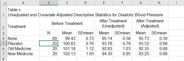
What's interesting about this table is that the posttest means are hardly adjusted by including our covariate. However, the covariate greatly reduces the standard errors for these means. This is why the mean differences are statistically significant only when the covariate is included. The adjusted descriptives are obtained from the final ANCOVA results. The unadjusted descriptives can be created from the syntax below.
means predias postdias by treatment
/cells count mean semean.
The exact APA table is best created by copy-pasting these statistics into Excel or Googlesheets.
Second, we'll present a standard ANOVA table for the effects included in our final model and error.
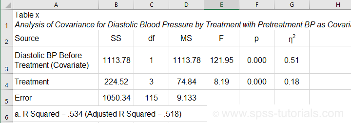
This table is constructed by copy-pasting the SPSS output table into Excel and removing the redundant rows.
Final Notes
So that'll do for a very solid but simple ANCOVA in SPSS. We could have written way more about this example analysis as there's much -much- more to say about the output. We'd also like to cover the basic ideas behind ANCOVA into more detail but that really requires a separate tutorial which we hope to write in some weeks from now.
Hope my tutorial has been helpful anyway. So last off:
thanks for reading!
THIS TUTORIAL HAS 24 COMMENTS:
By Joel Azuure Adongo on June 9th, 2022
Very helpful. Thanks
By Tim Kelly on August 8th, 2022
Excellent tutorial - thanks!
By Peter Paul on October 31st, 2022
Thank you for posting these helpful tutorials. These help me further.
You mention: "We now run simply rerun our ANCOVA as previously. This time, however, we'll remove the covariate by treatment interaction effect. "
I don't understand why I should run again the analysis, because in analysis 'ANCOVA I', all the required calculations are done. Therefore, it seems duplicitous to me to run it again, except the interaction. So, is it necessary to run 'ANCOVA II', and if so: why?
Thanks in advance.
Greetings,
Peter-Paul
By Ruben Geert van den Berg on November 1st, 2022
Hi Peter Paul!
For this particular example, it doesn't matter too much.
More generally, however, the idea is that you're just not interested in such interaction effects.
By adding them to your model, you lose degrees of freedom and -hence- power for testing the effects that you do find interesting.
It's a bit like adding tons of predictors from which you expect nothing to a multiple regression equation. This usually deteriorates -rather than improves- your final model: it becomes bloated and you may see adjusted r-square decrease as you add more useless predictors.
Hope that helps!
Ruben Geert van den Berg
SPSS tutorials
By Peter Paul van der Ven on November 2nd, 2022
Dear Ruben Geert,
Thank you for your clear answer. This helps me further!
Greetings, Peter Paul