Effect Size – A Quick Guide

Effect size is an interpretable number that quantifies
the difference between data and some hypothesis.

• Overview Effect Size Measures
• Chi-Square Tests
• T-Tests
• Pearson Correlations
• ANOVA
• Linear Regression

Statistical significance is roughly the probability of finding your data if some hypothesis is true. If this probability is low, then this hypothesis probably wasn't true after all. This may be a nice first step, but what we really need to know is how much do the data differ from the hypothesis? An effect size measure summarizes the answer in a single, interpretable number. This is important because

1. effect sizes allow us to compare effects -both within and across studies;
2. we need an effect size measure to estimate (1 - β) or power. This is the probability of rejecting some null hypothesis given some alternative hypothesis;
3. even before collecting any data, effect sizes tell us which sample sizes we need to obtain a given level of power -often 0.80.

Overview Effect Size Measures

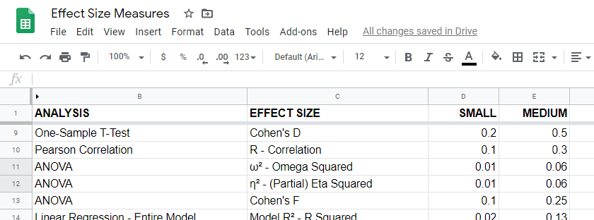
For an overview of effect size measures, please consult this Googlesheet shown below. This Googlesheet is read-only but can be downloaded and shared as Excel for sorting, filtering and editing.

Chi-Square Tests

Common effect size measures for chi-square tests are

• Cohen’s W (both chi-square tests);
• Cramér’s V (chi-square independence test) and
• the contingency coefficient (chi-square independence test) .

Chi-Square Tests - Cohen’s W

Cohen’s W is the effect size measure of choice for

• the chi-square independence test and
• the chi-square goodness-of-fit test.

Basic rules of thumb for Cohen’s W⁸ are

• small effect: w = 0.10;
• medium effect: w = 0.30;
• large effect: w = 0.50.

Cohen’s W is computed as

$$W = \sqrt{\sum_{i = 1}^m\frac{(P_{oi} - P_{ei})^2}{P_{ei}}}$$

where

• \(P_{oi}\) denotes observed proportions and
• \(P_{ei}\) denotes expected proportions under the null hypothesis for
• \(m\) cells.

For contingency tables, Cohen’s W can also be computed from the contingency coefficient \(C\) as

$$W = \sqrt{\frac{C^2}{1 - C^2}}$$

A third option for contingency tables is to compute Cohen’s W from Cramér’s V as

$$W = V \sqrt{d_{min} - 1}$$

where

• \(V\) denotes Cramér's V and
• \(d_{min}\) denotes the smallest table dimension -either the number of rows or columns.

Cohen’s W is not available from any statistical packages we know. For contingency tables, we recommend computing it from the aforementioned contingency coefficient.

For chi-square goodness-of-fit tests for frequency distributions your best option is probably to compute it manually in some spreadsheet editor. An example calculation is presented in this Googlesheet.

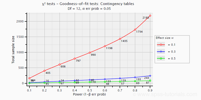
Power and required sample sizes for chi-square tests can't be directly computed from Cohen’s W: they depend on the df -short for degrees of freedom- for the test. The example chart below applies to a 5 · 4 table, hence df = (5 - 1) · (4 -1) = 12.

T-Tests

Common effect size measures for t-tests are

• Cohen’s D (all t-tests) and
• the point-biserial correlation (only independent samples t-test).

T-Tests - Cohen’s D

Cohen’s D is the effect size measure of choice for all 3 t-tests:

• the independent samples t-test,
• the paired samples t-test and
• the one sample t-test.

Basic rules of thumb are that⁸

• |d| = 0.20 indicates a small effect;
• |d| = 0.50 indicates a medium effect;
• |d| = 0.80 indicates a large effect.

For an independent-samples t-test, Cohen’s D is computed as

$$D = \frac{M_1 - M_2}{S_p}$$

where

• \(M_1\) and \(M_2\) denote the sample means for groups 1 and 2 and
• \(S_p\) denotes the pooled estimated population standard deviation.

A paired-samples t-test is technically a one-sample t-test on difference scores. For this test, Cohen’s D is computed as

$$D = \frac{M - \mu_0}{S}$$

where

• \(M\) denotes the sample mean,
• \(\mu_0\) denotes the hypothesized population mean (difference) and
• \(S\) denotes the estimated population standard deviation.

Cohen’s D is present in JASP as well as SPSS (version 27 onwards). For a thorough tutorial, please consult Cohen’s D - Effect Size for T-Tests.

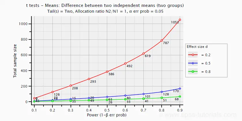
The chart below shows how power and required total sample size are related to Cohen’s D. It applies to an independent-samples t-test where both sample sizes are equal.

Pearson Correlations

For a Pearson correlation, the correlation itself (often denoted as r) is interpretable as an effect size measure. Basic rules of thumb are that⁸

• r = 0.10 indicates a small effect;
• r = 0.30 indicates a medium effect;
• r = 0.50 indicates a large effect.

Pearson correlations are available from all statistical packages and spreadsheet editors including Excel and Google sheets.

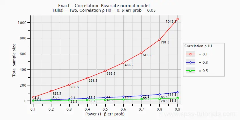
The chart below -created in G*Power- shows how required sample size and power are related to effect size.

ANOVA

Common effect size measures for ANOVA are

• \(\color{#0a93cd}{\eta^2}\) or (partial) eta squared;
• Cohen’s F;
• \(\color{#0a93cd}{\omega^2}\) or omega-squared.

ANOVA - (Partial) Eta Squared

Partial eta squared -denoted as η²- is the effect size of choice for

• ANOVA (between-subjects, one-way or factorial);
• repeated measures ANOVA (one-way or factorial);
• mixed ANOVA.

Basic rules of thumb are that

• η² = 0.01 indicates a small effect;
• η² = 0.06 indicates a medium effect;
• η² = 0.14 indicates a large effect.

Partial eta squared is calculated as

$$\eta^2_p = \frac{SS_{effect}}{SS_{effect} + SS_{error}}$$

where

• \(\eta^2_p\) denotes partial eta-squared and
• \(SS\) denotes effect and error sums of squares.

This formula also applies to one-way ANOVA, in which case partial eta squared is equal to eta squared.

Partial eta squared is available in all statistical packages we know, including JASP and SPSS. For the latter, see How to Get (Partial) Eta Squared from SPSS?

ANOVA - Cohen’s F

Cohen’s f is an effect size measure for

• ANOVA (between-subjects, one-way or factorial);
• repeated measures ANOVA (one-way or factorial);
• mixed ANOVA.

Cohen’s f is computed as

$$f = \sqrt{\frac{\eta^2_p}{1 - \eta^2_p}}$$

where \(\eta^2_p\) denotes (partial) eta-squared.

Basic rules of thumb for Cohen’s f are that⁸

• f = 0.10 indicates a small effect;
• f = 0.25 indicates a medium effect;
• f = 0.40 indicates a large effect.

G*Power computes Cohen’s f from various other measures. We're not aware of any other software packages that compute Cohen’s f.

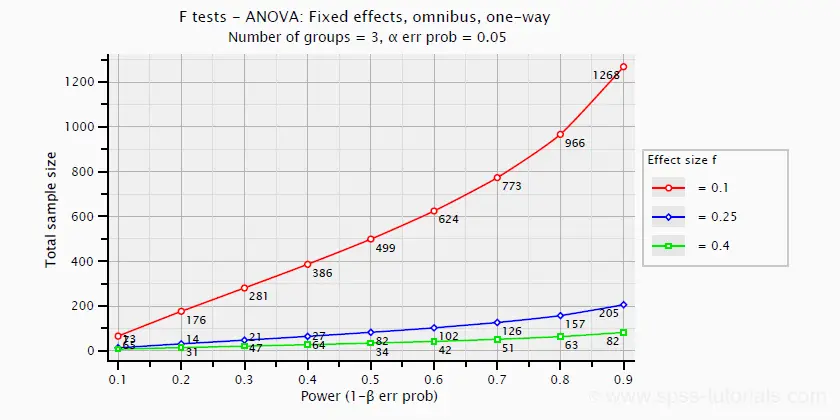
Power and required sample sizes for ANOVA can be computed from Cohen’s f and some other parameters. The example chart below shows how required sample size relates to power for small, medium and large effect sizes. It applies to a one-way ANOVA on 3 equally large groups.

ANOVA - Omega Squared

A less common but better alternative for (partial) eta-squared is \(\omega^2\) or Omega squared computed as

$$\omega^2 = \frac{SS_{effect} - df_{effect}\cdot MS_{error}}{SS_{total} + MS_{error}}$$

where

• \(SS\) denotes sums of squares;
• \(df\) denotes degrees of freedom;
• \(MS\) denotes mean squares.

Similarly to (partial) eta squared, \(\omega^2\) estimates which proportion of variance in the outcome variable is accounted for by an effect in the entire population. The latter, however, is a less biased estimator.^1,2,6 Basic rules of thumb are⁵

• Small effect: ω² = 0.01;
• Medium effect: ω² = 0.06;
• Large effect: ω² = 0.14.

\(\omega^2\) is available in SPSS version 27 onwards but only if you run your ANOVA from Analyze Compare Means One-Way ANOVA The other ANOVA options in SPSS (via General Linear Model or Means) do not yet include \(\omega^2\). However, it's also calculated pretty easily by copying a standard ANOVA table into Excel and entering the formula(s) manually.

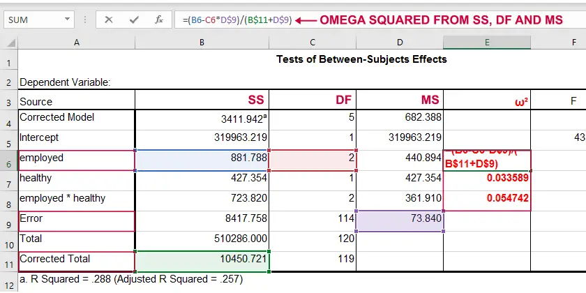Note: you need “Corrected total” for computing omega-squared from SPSS output.

Linear Regression

Effect size measures for (simple and multiple) linear regression are

• \(\color{#0a93cd}{f^2}\) (entire model and individual predictor);
• \(R^2\) (entire model);
• \(r_{part}^2\) -squared semipartial (or “part”) correlation (individual predictor).

Linear Regression - F-Squared

The effect size measure of choice for (simple and multiple) linear regression is \(f^2\). Basic rules of thumb are that⁸

• \(f^2\) = 0.02 indicates a small effect;
• \(f^2\) = 0.15 indicates a medium effect;
• \(f^2\) = 0.35 indicates a large effect.

\(f^2\) is calculated as

$$f^2 = \frac{R_{inc}^2}{1 - R_{inc}^2}$$

where \(R_{inc}^2\) denotes the increase in r-square for a set of predictors over another set of predictors. Both an entire multiple regression model and an individual predictor are special cases of this general formula.

For an entire model, \(R_{inc}^2\) is the r-square increase for the predictors in the model over an empty set of predictors. Without any predictors, we estimate the grand mean of the dependent variable for each observation and we have \(R^2 = 0\). In this case, \(R_{inc}^2 = R^2_{model} - 0 = R^2_{model}\) -the “normal” r-square for a multiple regression model.

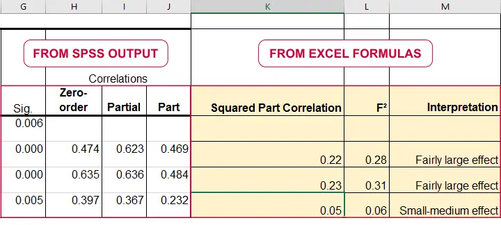
For an individual predictor, \(R_{inc}^2\) is the r-square increase resulting from adding this predictor to the other predictor(s) already in the model. It is equal to \(r^2_{part}\) -the squared semipartial (or “part”) correlation for some predictor. This makes it very easy to compute \(f^2\) for individual predictors in Excel as shown below.

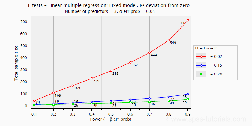
\(f^2\) is useful for computing the power and/or required sample size for a regression model or individual predictor. However, these also depend on the number of predictors involved. The figure below shows how required sample size depends on required power and estimated (population) effect size for a multiple regression model with 3 predictors.

Right, I think that should do for now. We deliberately limited this tutorial to the most important effect size measures in a (perhaps futile) attempt to not overwhelm our readers. If we missed something crucial, please throw us a comment below. Other than that,

thanks for reading!

References

1. Van den Brink, W.P. & Koele, P. (2002). Statistiek, deel 3 [Statistics, part 3]. Amsterdam: Boom.
2. Warner, R.M. (2013). Applied Statistics (2nd. Edition). Thousand Oaks, CA: SAGE.
3. Agresti, A. & Franklin, C. (2014). Statistics. The Art & Science of Learning from Data. Essex: Pearson Education Limited.
4. Hair, J.F., Black, W.C., Babin, B.J. et al (2006). Multivariate Data Analysis. New Jersey: Pearson Prentice Hall.
5. Field, A. (2013). Discovering Statistics with IBM SPSS Statistics. Newbury Park, CA: Sage.
6. Howell, D.C. (2002). Statistical Methods for Psychology (5th ed.). Pacific Grove CA: Duxbury.
7. Siegel, S. & Castellan, N.J. (1989). Nonparametric Statistics for the Behavioral Sciences (2nd ed.). Singapore: McGraw-Hill.
8. Cohen, J (1988). Statistical Power Analysis for the Social Sciences (2nd. Edition). Hillsdale, New Jersey, Lawrence Erlbaum Associates.
9. Pituch, K.A. & Stevens, J.P. (2016). Applied Multivariate Statistics for the Social Sciences (6th. Edition). New York: Routledge.

How to Get (Partial) Eta Squared from SPSS?

In ANOVA, we always report

• F (the F-value);
• df (degrees of freedom);
• p (statistical significance).

We report these 3 numbers for each effect -possibly just one for one-way ANOVA. Now, p (“Sig.” in SPSS) tells us the likelihood of some effect being zero in our population. A zero effect means that all means are exactly equal for some factor such as gender or experimental group.

However, some effect just being not zero isn't too interesting, is it? What we really want to know is: how strong is the effect? We can't conclude that p = 0.05 indicates a stronger effect than p = 0.10 because both are affected by sample sizes and other factors. So how can we quantify how strong effects are for comparing them within or across analyses?
Well, there's several measures of effect size that tell us just that. One that's often used is (partial) eta squared, denoted as η² (η is the Greek letter eta).

Partial Eta Squared - What Is It?

Partial η² a proportion of variance accounted for by some effect. If you really really want to know: $$partial\;\eta^2 = \frac{SS_{effect}}{SS_{effect} + SS_{error}}$$
where SS is short for “sums of squares”, the amount of dispersion in our dependent variable. This means that partial η² is the variance attributable to an effect divided by the variance that could have been attributable to this effect.
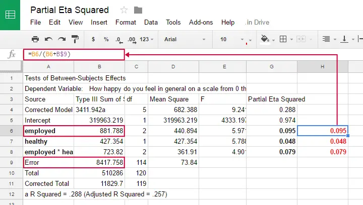
We can easily verify this -and many more calculations- by copy-pasting SPSS’ ANOVA output into this GoogleSheet as shown below.

Note that in one-way ANOVA, we only have one effect. So the variance in our dependent variable is either attributed to the effect or it is error. So for one-way ANOVA $$partial\;\eta^2 = \frac{SS_{effect}}{SS_{total}}$$
which is equal to (non partial) η². Let's now go and get (partial) η² from SPSS.

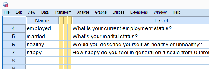
Example: Happiness Study

A scientist asked 120 people to rate their own happiness on a 100 point scale. Some other questions were employment status, marital status and health. The data thus collected are in happy.sav, part of which is shown below.

We're especially interested in the effect of employment on happiness: (how) are they associated and does the association depend on health or marital status too? Let's first just examine employment with a one-way ANOVA.

Eta Squared for One-Way ANOVA - Option 1

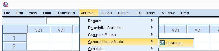
SPSS offers several options for running a one-way ANOVA and many students start off with Analyze Compare Means One-Way ANOVA but -oddly- η² is completely absent from this dialog.
We'll therefore use MEANS instead as shown below.

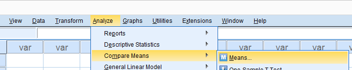
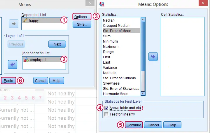
Clicking Paste results in the syntax below. Since it's way longer than necessary, I prefer just typing a short version that yields identical results. Let's run it.

SPSS Syntax for Eta Squared from MEANS

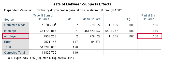
Result

And there we have it: η² = 0.166: some 17% of all variance in happiness is attributable to employment status. I'd say it's not an awful lot but certainly not negligible.
Note that SPSS mentions “Measures of Association” rather than “effect size”. It could be argued that these are interchangeable but it's somewhat inconsistent anyway.

Eta Squared for One-Way ANOVA - Option 2

Perhaps the best way to run ANOVA in SPSS is from the univariate GLM dialog. The screenshots below guide you through.

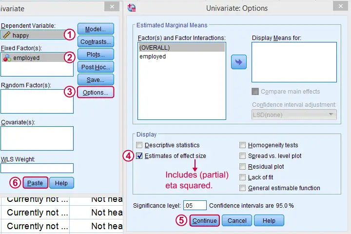
This results in the syntax shown below. Let's run it, see what happens.

SPSS Syntax for Eta Squared from UNIANOVA

Result

We find partial η² = 0.166. It was previously denoted as just η² but these are identical for one-way ANOVA as already discussed.

Partial Eta Squared for Multiway ANOVA

For multiway ANOVA -involving more than 1 factor- we can get partial η² from GLM univariate as shown below.

As shown below, we now just add multiple independent variables (“fixed factors”). We then tick Estimates of effect size under Options and we're good to go.

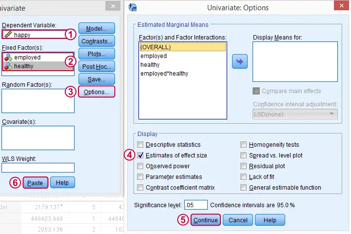
Partial Eta Squared Syntax Example

Result

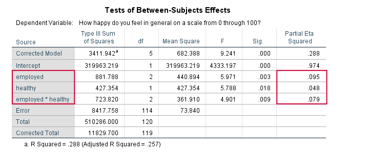
First off, both main effects (employment and health) and the interaction between them are statistically significant. The effect of employment (η² = .095) is twice as strong as health (η² = 0.048). And so on.
Note that you couldn't possibly conclude this from their p-values (p = 0.003 for employment and p = 0.018 for health). Although the effects are highly statistically significant, the effect sizes are moderate. We typically see this pattern with larger sample sizes.
Last, we shouldn't really interpret our main effects because the interaction effect is statistically significant: F(2,114) = 4.9, p = 0.009. As explained in SPSS Two Way ANOVA - Basics Tutorial, we'd better inspect simple effects instead of main effects.

Conclusion

We can get (partial) η² for both one-way and multiway ANOVA from Analyze General Linear Model Univariate but it's restricted to one dependent variable at the time. Generally, I'd say this is the way to go for any ANOVA because it's the only option that gets us all the output we generally need -including post hoc tests and Levene's test.

We can run multiple one-way ANOVAs with η² in one go with Analyze Compare Means Means but it lacks important options such as post hoc tests and Levene's test. These -but not η² - are available from the One-Way ANOVA dialog. This renders both options rather inconvenient unless you need a very basic analysis.

Last, several authors prefer a different measure of effect size called ω² (“Omega square”). Unfortunately, this seems completely absent from SPSS. For now at least, I guess η² will have to do...

I hope you found this tutorial helpful. Thanks for reading!