SPSS Z-Test for a Single Proportion

• Z-Test - Assumptions
• SPSS Z-Test Dialogs
• SPSS Z-Test Output
• APA Style Reporting Z-Tests
• References

A z-test for a single proportion tests
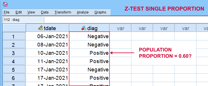
if some population proportion is equal to x. Example: does a proportion of 0.60 (or 60%) of all Dutch citizens test positive on Covid-19?

In order to find out, a scientist tested a simple random sample of N = 112 people. The results thus gathered are in covid-z-test.sav, partly shown below.

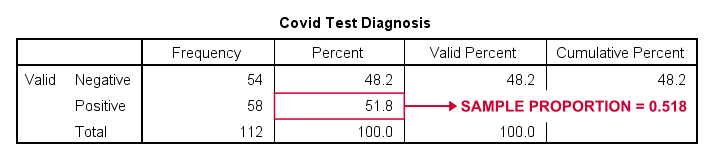
The first thing we'd like to know is: what's our sample proportion anyway? We'll quickly find out by running a single line of SPSS syntax: frequencies diag. The resulting table tells us that 51.8% (a proportion of .518) of our sample tested positive on Covid-19.

Now, does our sample outcome of 51.8% really contradict our null hypothesis that 60% of our entire population is infected? A z-test for a single proportion answers just that. However, it does require a couple of assumptions.

Z-Test - Assumptions

A z-test for a single proportion requires two assumptions:

• independent observations;
• \(n_1 \ge 15\) and \(n_2 \ge 15\): our sample should contain at least some 15 observations for either possible outcome.

Standard textbooks^3,5 often propose \(n_1 \ge 5\) and \(n_2 \ge 5\) but recent studies suggest that these sample sizes are insufficient for accurate test results.² For small sample sizes, the Agresti-Coull adjustment may somewhat improve your results.

A quick check for the sample sizes assumption is inspecting basic frequency distributions for the outcome variables. We already did this for our example data. Our outcomes -Covid negative or positive- have frequencies of 54 and 58 observations.

SPSS Z-Test Dialogs

Starting from SPSS version 27, z-tests are found under Analyze Compare Means One-Sample Proportions For our example study, we'll fill in the dialogs as shown below.

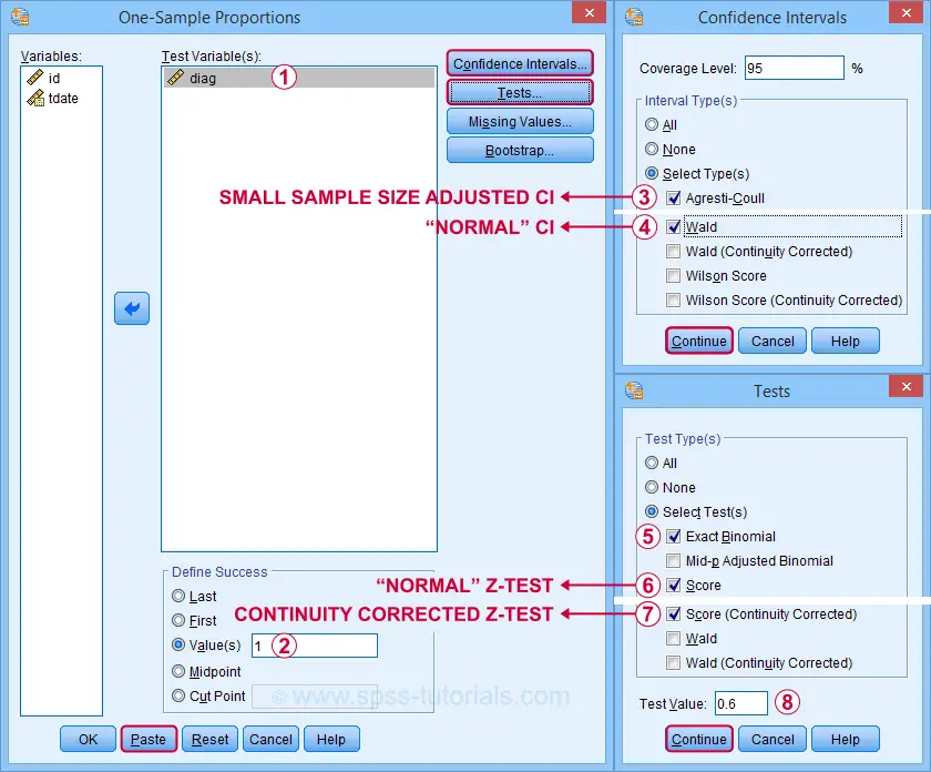
Our hypothesis addresses the proportion of positive tests, which is coded as 1 in our data.
Precisely, we hypothesized a population proportion of 0.60 (or 60%) to test positive for Covid-19.

Selecting these options results in the syntax below. Let's run it.

SPSS Z-Test Output

The first output table presents 95% confidence intervals for our population proportion.

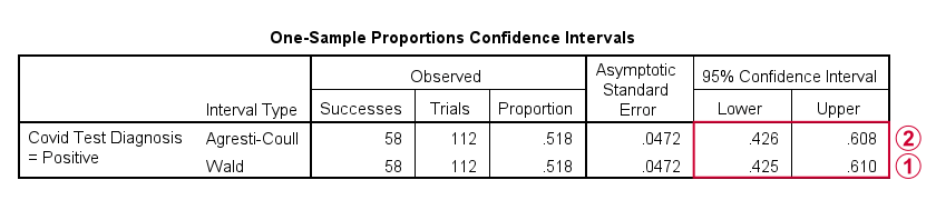
The “normal” confidence interval (denoted as Wald) runs from .425 to .610: there's a 95% probability that these bounds enclose our population proportion. Also note that our hypothesized proportion of .60 lies within this interval of likely values.

The Agresti-Coull interval is probably a worse estimate than our “normal” confidence interval unless the sample sizes assumption is not met. I recommend ignoring it for our example data.

The second table presents the actual z-test results.

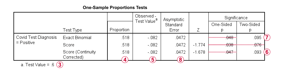
Our hypothesized population proportion is .60.
Our observed sample proportion is .518.
The observed difference is .518 - .60 = -.082.

The continuity corrected significance level is always more accurate than the uncorrected p-value. For our example, p(2-tailed) = .093. Because p > .05, we do not reject the null hypothesis that our population proportion = .60. That is, the difference of -.082 is not statistically significant.

The binomial test yields an exact 1-tailed p-value. Its 2-tailed p-value, however, is not correct: it's exactly 2 * p(1-tailed) but this calculation is only valid if the test proportion is 0.50.

For test proportions other than 0.50, the binomial distribution is asymmetrical. This is why the “traditional” binomial test in SPSS doesn't report any p(2-tailed) in this case as can be verified by the syntax below.

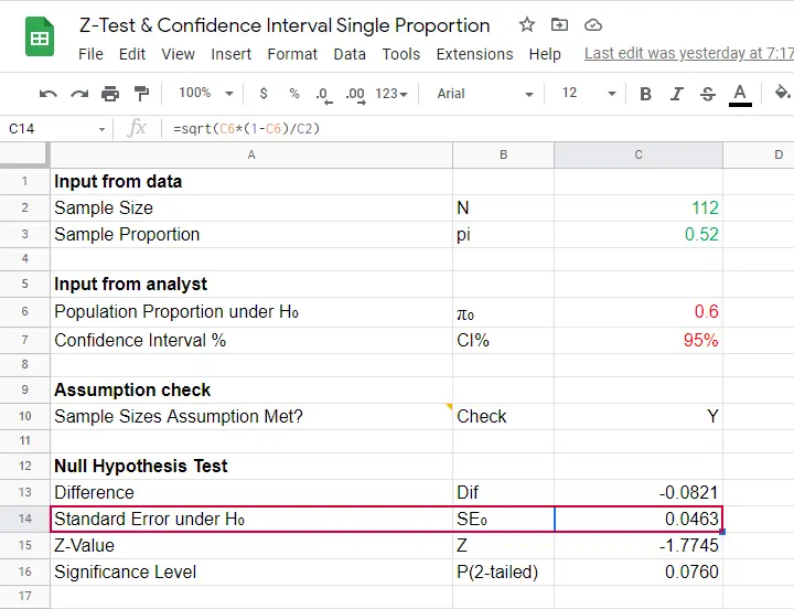
Finally, note that SPSS reports the wrong standard error. The correct standard error is .0463 as computed in this Googlesheet (read-only).

APA Style Reporting Z-Tests

The APA does not have explicit guidelines on reporting z-tests. However, it makes sense to report something like “the proportion of positive Covid-19 diagnoses did not differ significantly from 0.60, z = -1.68, p(2-tailed) = .093.” Obviously, you should also report

• your sample size;
• the observed sample proportion;
• whether the continuity correction was applied to the z-test;
• whether the Agresti-Coull correction was applied to the confidence interval.

Final Notes

Altogether, I think z-tests are rather poorly implemented in SPSS:

• the standard error for the z-test is not correct;
• p(2-tailed) for the binomial test is not correct;
• no warning is issued if sample sizes are even way insufficient to run a z-test in the first place;
• no effect size measures (such as Cohen’s H) are available;
• z-tests and confidence intervals are reported in separate tables which the end user will probably want to merge in Excel or something.

What's really good, however, is that

• z-tests in SPSS handle (even a combination of) numeric and string variables;
• several corrections for both the z-test and confidence intervals are available.

Thanks for reading!

References

1. Agresti, A. & Coull, B.A. (1998). Approximate Is Better than "Exact" for Interval Estimation of Binomial Proportions The American Statistician, 52(2), 119-126.
2. Agresti, A. & Franklin, C. (2014). Statistics. The Art & Science of Learning from Data. Essex: Pearson Education Limited.
3. Van den Brink, W.P. & Koele, P. (1998). Statistiek, deel 2 [Statistics, part 2]. Amsterdam: Boom.
4. Van den Brink, W.P. & Koele, P. (2002). Statistiek, deel 3 [Statistics, part 3]. Amsterdam: Boom.
5. Twisk, J.W.R. (2016). Inleiding in de Toegepaste Biostatistiek [Introduction to Applied Biostatistics]. Houten: Bohn Stafleu van Loghum.

SPSS Sign Test for One Median – Simple Example

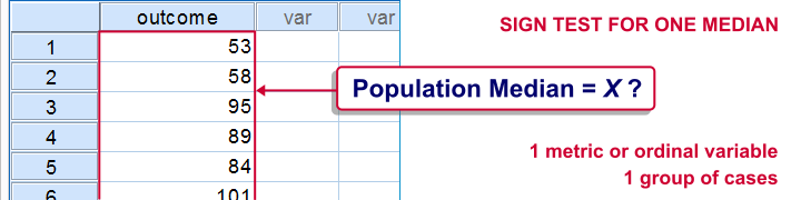
A sign test for one median is often used instead of a one sample t-test when the latter’s assumptions aren't met by the data. The most common scenario is analyzing a variable which doesn't seem normally distributed with few (say n < 30) observations. For larger sample sizes the central limit theorem ensures that the sampling distribution of the mean will be normally distributed regardless of how the data values themselves are distributed.
This tutorial shows how to run and interpret a sign test in SPSS. We'll use adratings.sav throughout, part of which is shown below.

SPSS Sign Test - Null Hypothesis

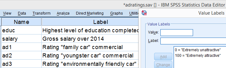
A car manufacturer had 3 commercials rated on attractiveness by 18 people. They used a percent scale running from 0 (extremely unattractive) through 100 (extremely attractive). A marketeer thinks a commercial is good if at least 50% of some target population rate it 80 or higher.
Now, the score that divides the 50% lowest from the 50% highest scores is known as the median. In other words, 50% of the population scoring 80 or higher is equivalent to our null hypothesis that the population median is at least 79.5 for each commercial. If this is true, then the medians in our sample will be somewhat different due to random sampling fluctuation. However, if we find very different medians in our sample, then our hypothesized 79.5 population median is not credible and we'll reject our null hypothesis.

Quick Data Check - Histograms

Let's first take a quick look at what our data look like in the first place. We'll do so by inspecting histograms over our outcome variables by running the syntax below.

Result

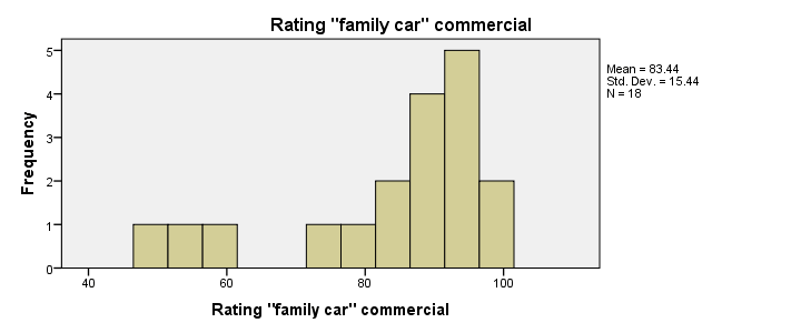
First, note that all distributions look plausible. Since n = 18 for each variable, we don't have any missing values. The distributions don't look much like normal distributions. Combined with our small sample sizes, this violates the normality assumption required by t-tests so we probably shouldn't run those.

Quick Data Check - Medians

Our histograms included mean scores for our 3 outcome variables but what about their medians? Very oddly, we can't compute medians -which are descriptive statistics- with DESCRIPTIVES. We could use FREQUENCIES but we prefer the table format we get from MEANS as shown below.

SPSS - Compute Medians Syntax

Result

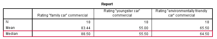
Only our first commercial (“family car”) has a median close to 79.5. The other 2 commercials have much lower median. But are they different enough for rejecting our null hypothesis? We'll find out in a minute.

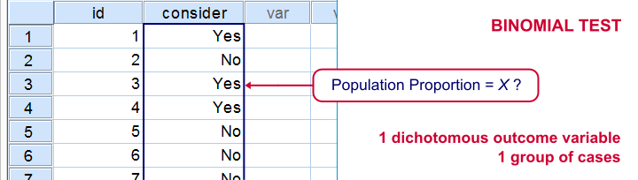
SPSS Sign Test - Recoding Data Values

SPSS includes a sign test for two related medians but the sign test for one median is absent. But remember that our null hypothesis of a 79.5 population median is equivalent to 50% of the population scoring 80 or higher. And SPSS does include a test for a single proportion (a percentage divided by 100) known as the binomial test. We'll therefore just use binomial tests for evaluating if the proportion of respondents rating each commercial 80 or higher is equal to 0.50.
The easy way to go here is to RECODE our data values: values smaller than the hypothesized population median are recoded into a minus (-) sign. Values larger than this median get a plus (+) sign. It's these plus and minus signs that give the sign test its name. Values equal to the median are excluded from analysis so we'll specify them as missing values.

SPSS RECODE Syntax

SPSS Binomial Test Menu

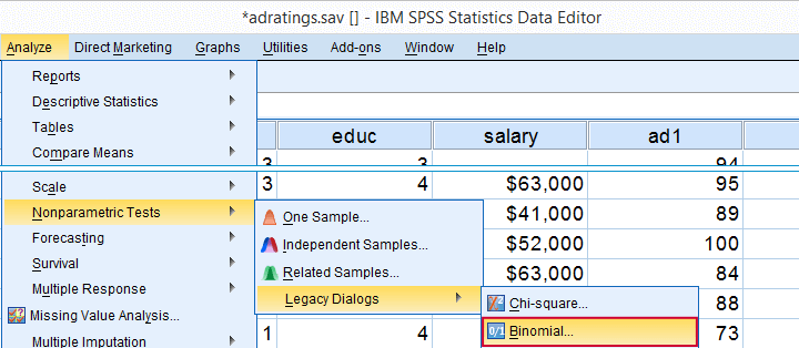
Minor note: the binomial test is a test for a single proportion, which is a population parameter. So it's clearly not a nonparametric test. Unfortunately, “nonparametric tests” often refers to both nonparametric and distribution free tests -even though these are completely different things.

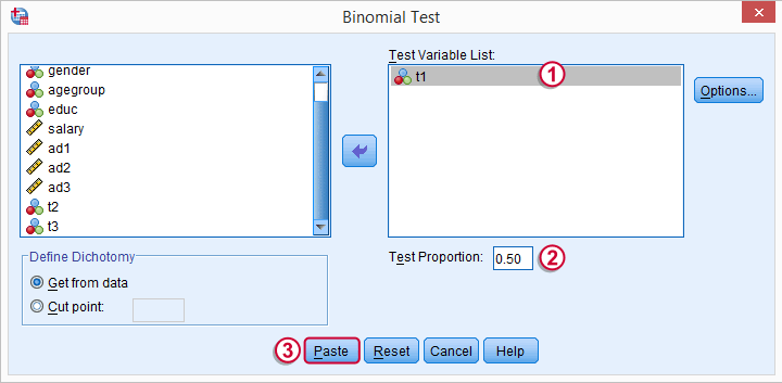
t1 is one of our newly created variables. It merely indicates if ad1 was 80 or higher. Completing the steps results in the syntax below.

SPSS Binomial Test Syntax

Modifying Our Syntax

Oddly, SPSS’ binomial test results depend on the (arbitrary) order of cases: the test proportion applies to the first value encountered in the data. This is no major issue if -and only if- our test proportion is 0.50 but it still results in messy output. We'll avoid this by sorting our cases on each test variable before each test.

Modified Binomial Test Syntax

Binomial Test Output

We'll first limit our focus to the first table of test results as shown below.

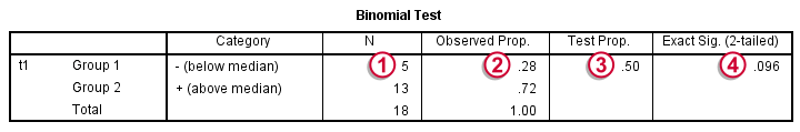
N: 5 out of 18 cases score higher than 79.5;
the observed proportion is (5 / 18 =) 0.28 or 28%;
the hypothesized test proportion is 0.50;
p (denoted as “Exact Significance (2-tailed)”) = 0.096: the probability of finding our sample result is roughly 10% if the population proportion really is 50%. We generally reject our null hypothesis if p < 0.05 so our binomial test does not refute the hypothesis that our population median is 79.5. Before we move on, let's take a close look at what our 2-tailed p-value of 0.096 really means.

The Binomial Distribution

Statistically, drawing 18 respondents from a population in which 50% scores 80 or higher is similar to flipping a balanced coin 18 times in a row: we could flip anything between 0 and 18 heads. If we repeat our 18 coin flips over and over again, the sampling distribution of the number of heads will closely resemble the binomial distribution shown below.

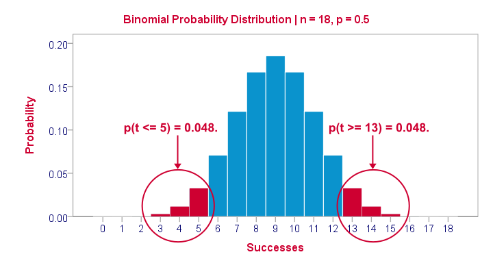
The most likely outcome is 9 heads with a probability around 0.19 or 19%. P = 0.048 for outcomes of 5 or fewer heads (red area). Now, reporting this 1-tailed p-value suggests that none of the other outcomes would refute the null hypothesis. This does not hold because 13 or more heads are also highly unlikely. So we should take into account our deviation of 4 heads from the expected 9 heads in both directions and add up their probabilities. This results in our 2-tailed p-value of 0.096.

Binomial Test - More Output

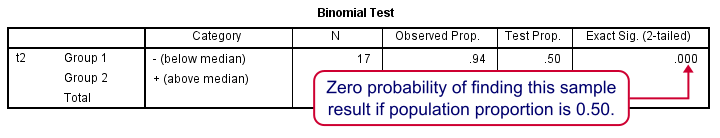
We saw previously that our second commercial (“youngster car”) has a sample median of 55.5. Our p-value of 0.000 means that we've a 0% probability of finding this sample median in a sample of n = 18 when the population median is 79.5. Since p < 0.05, we reject the null hypothesis: the population median is not 79.5 but -presumably- much lower. We'll leave it as an exercise to the reader to interpret the third and final test.

That's it for now. I hope this tutorial made clear how to run a sign test for one median in SPSS. Please let us know what you think in the comment section below. Thanks!

Binomial Test – Simple Tutorial

For running a binomial test in SPSS, see SPSS Binomial Test.

A binomial test examines if some
population proportion is likely to be x. For example, is 50% -a proportion of 0.50- of the entire Dutch population familiar with my brand? We asked a simple random sample of N = 10 people if they are. Only 2 of those -a proportion of 0.2- or 20% know my brand. Does this sample proportion of 0.2 mean that the population proportion is not 0.5? Or is 2 out of 10 a pretty normal outcome if 50% of my population really does know my brand?
The binomial test is the simplest statistical test there is. Understanding how it works is pretty easy and will help you understand other statistical significance tests more easily too. So how does it work?

Binomial Test - Basic Idea

If the population proportion really is 0.5, we can find a sample proportion of 0.2. However, if the population proportion is only 0.1 (only 10% of all Dutch adults know the brand), then we may also find a sample proportion of 0.2. Or 0.9. Or basically any number between 0 and 1. The figure below illustrates the basic problem -I mean challenge- here.

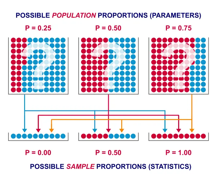Will the real population proportion please stand up now??

So how can we conclude anything at all about our population based on just a sample? Well, we first make an initial guess about the population proportion which we call the null hypothesis: a population proportion of 0.5 knows my brand.
Given this hypothesis, many sample proportions are possible. However, some outcomes are extremely unlikely or almost impossible. If we do find an outcome that's almost impossible given some hypothesis, then the hypothesis was probably wrong: we conclude that the population proportion wasn't x after all.
So that's how we draw population conclusions based on sample outcomes. Basically all statistical tests follow this line of reasoning. The basic question for now is: what's the probability of finding 2 successes in a sample of 10 if the population proportion is 0.5?

Binomial Test Assumptions

First off, we need to assume independent observations. This basically means that the answer given by any respondent must be independent of the answer given by any other respondent. This assumption (required by almost all statistical tests) has been met by our data.

Binomial Distribution - Formula

If 50% of some population knows my brand and I ask 10 people, then my sample could hold anything between 0 and 10 successes. Each of these 11 possible outcomes and their associated probabilities are an example of a binomial distribution, which is defined as $$P(B = k) = \binom{n}{k} p^k (1 - p)^{n - k}$$ where

• \(n\) is the number of trials (sample size);
• \(k\) is the number of successes;
• \(p\) is the probability of success for a single trial or the (hypothesized) population proportion.

Note that \(\binom{n}{k}\) is a shorthand for \(\frac{n!}{k!(n - k)!}\) where \(!\) indicates a factorial.

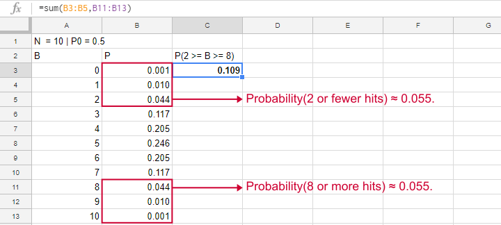
For practical purposes, we get our probabilities straight from Google Sheets (it uses the aforementioned formula under the hood but it doesn't bother us with it).

Binomial Distribution - Chart

Right, so we got the probabilities for our 11 possible outcomes (0 through 10 successes) and visualized them below.

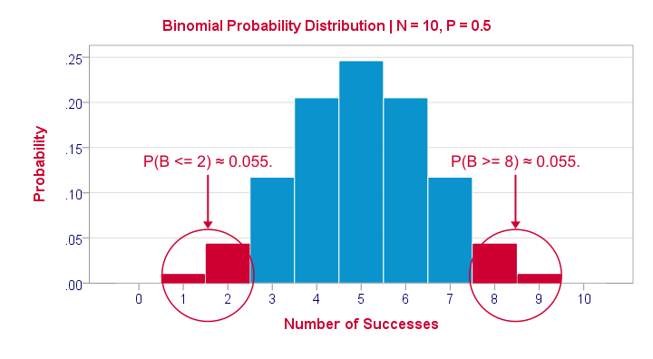
If a population proportion is 0.5 and we sample 10 observations, the most likely outcome is 5 successes: P(B = 5) ≈ 0.24. Either 4 or 6 successes are also likely outcomes (P ≈ 0.2 for each).
The probability of finding 2 or fewer successes -like we did- is 0.055. This is our one-sided p-value.
Now, very low or very high numbers of successes are both unlikely outcomes and should both cast doubt on our null hypothesis. We therefore take into account the p-value for the opposite outcome -8 or more successes- which is another 0.055. Like so, we find a 2-sided p-value of 0.11. If we would draw 1,000 samples instead of just 1, then some 11% of those should result in 2(-) or 8(+) successes when the population proportion is 0.5. Our sample outcome should occur in a reasonable percentage of samples. And since 11% is not very unlikely, our sample does not refute our hypothesis that 50% of our population knows our brand.

Binomial Test - Google Sheets

We ran our example in this simple Google Sheet. It's accessible to anybody so feel free to take a look at it.

Binomial Test - SPSS

Perhaps the easiest way to run a binomial test is in SPSS - for a nice tutorial, try SPSS Binomial Test. The figure below shows the output for our current example. It obviously returns the same p-value of 0.109 as our Google Sheet.

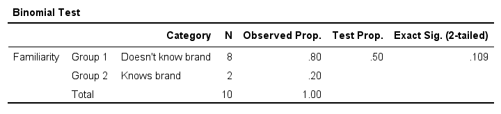
Note that SPSS refers to p as “Exact Sig. (2-tailed)”. Is there a non exact p-value too then? Well, sort of. Let's see how that works.

Binomial Test or Z Test?

Let's take another look at the binomial probability distribution we saw earlier. It kinda resembles a normal distribution. Not convinced? Take a look at the binomial distribution below.

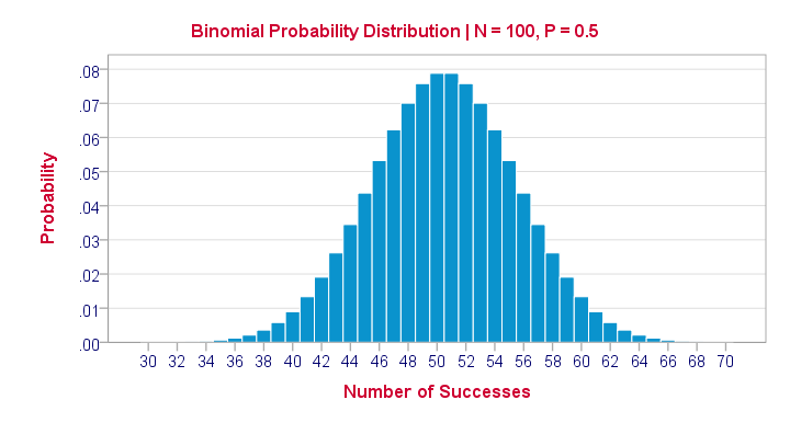
For a sample of N = 100, our binomial distribution is virtually identical to a normal distribution. This is caused by the central limit theorem. A consequence is that -for a larger sample size- a z-test for one proportion (using a standard normal distribution) will yield almost identical p-values as our binomial test (using a binomial distribution).

But why would we prefer a z-test over a binomial test?

• We can always use a 2-sided z-test. However, a binomial test is always 1-sided unless P₀ = 0.5.
• A z-test allows us to compute a confidence interval for our sample proportion.
• We can easily estimate statistical power for a z-test but not for a binomial test.
• A z-test is computationally less heavy, especially for larger sample sizes.I suspect that most software actually reports a z-test as if it were a binomial test for larger sample sizes.

So when can we use a z-test instead of a binomial test? A rule of thumb is that P₀*n and (1 - P₀)*n must both be > 5, where P₀ denotes the hypothesized population proportion and n the sample size.

So that's about it regarding the binomial test. I hope you found this tutorial helpful. Thanks for reading!

SPSS Binomial Test Tutorial

Also see Binomial Test - Simple Tutorial for a quick explanation of how this test works.

SPSS binomial test is used for testing whether a proportion from a single dichotomous variable is equal to a presumed population value. The figure illustrates the basic idea.

SPSS Binomial Test Example

A biologist claims that 75% of a population of spiders consist of female spiders. With a lot of effort he collects 15 spiders, 7 of which are female. These data are in spiders.sav, part of which are shown below.

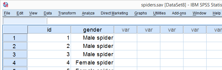
1. Quick Data Check

Let's first take a quick look at the FREQUENCIES for gender. Like so, we can inspect whether there are any missing values and whether the variable is really dichotomous. We'll run some FREQUENCIES. The syntax is so simple that we'll just type it instead of clicking through the menu.

The output tells us that there are no missing values and the variable is indeed dichotomous. We can proceed our analysis with confidence.

2. Assumptions Binomial Test

The results from any statistical test can only be taken seriously insofar as its assumptions have been met. For the binomial test we need just one:

• independent observations (or, more precisely, independent and identically distributed variables);

This assumption is beyond the scope of this tutorial. We presume it's been met by the data at hand.

3. Run SPSS Binomial Test

We'd like to test whether the proportion of female spiders differs from .75 (our test proportion). Now SPSS Binomial Test has a very odd feature: the test proportion we enter applies to the category that's first encountered in the data. So the hypothesis that's tested depends on the order of the cases. Because our test proportion applies to female (rather than male) spiders, we need to move our female spiders to the top of the data file. We'll do so by running the syntax below. Next, we'll run the actual binomial test.

Clicking Paste results in the syntax below. We'll run it and move on the output.

4. SPSS Binomial Test Output

Since we have 7 female spiders out of 15 observations, the observed proportion is (7 / 15 =) .47.
Our null hypothesis states that this proportion is .75 for the entire population.
The p value, denoted by Exact Sig. (1-tailed) is .017. If the proportion of female spiders is exactly .75 in the entire population, then there's only a 1.7% chance of finding 7 or fewer female spiders in a sample of N = 15. We often reject the null hypothesis if this chance is smaller than 5% (p < .05). We conclude that the proportion of female spiders is not .75 in the population but probably (much) lower.
Note that the p value is the chance of finding the observed proportion or a “more extreme” outcome. If the observed proportion is smaller than the test proportion, then a more extreme outcome is an even smaller proportion than the one we observe.The reasoning is entirely reversed when the observed proportion is larger than the expected proportion. We ignore the fact that finding very large proportions would also contradict our null hypothesis. This is what's meant by (1-tailed).A 2-tailed binomial test is only be applied when the test proportion is exactly .5. The (rather technical) reason for this is that the binomial sampling distribution for the observed proportion is only symmetrical in the latter case.

5. Reporting a Binomial Test

When reporting test results, we always report some descriptive statistics as well. In this case, a frequency table will do. Regarding the significance test, we'll write something like “a binomial test indicated that the proportion of female spiders of .47 was lower than the expected .75, p = .017 (1-sided)”.