Independent Samples T-Test – Quick Introduction

• Independent Samples T-Test - What Is It?
• Null Hypothesis
• Test Statistic
• Assumptions
• Statistical Significance
• Effect Size

Independent Samples T-Test - What Is It?

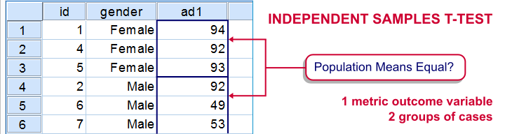
An independent samples t-test evaluates if 2 populations have equal means on some variable. If the population means are really equal, then the sample means will probably differ a little bit but not too much. Very different sample means are highly unlikely if the population means are equal. This sample outcome thus suggest that the population means weren't equal after all.
The samples are independent because they don't overlap; none of the observations belongs to both samples simultaneously. A textbook example is male versus female respondents.

Example

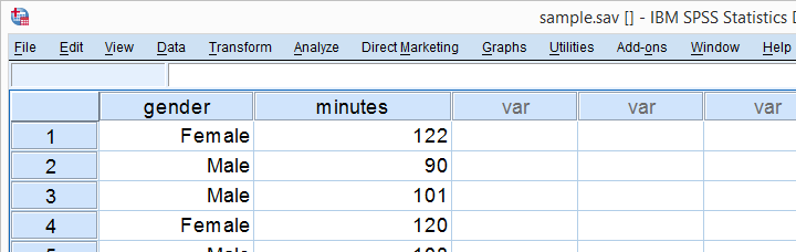
Some island has 1,000 male and 1,000 female inhabitants. An investigator wants to know if males spend more or fewer minutes on the phone each month. Ideally, he'd ask all 2,000 inhabitants but this takes too much time. So he samples 10 males and 10 females and asks them. Part of the data are shown below.

Next, he computes the means and standard deviations of monthly phone minutes for male and female respondents separately. The results are shown below.

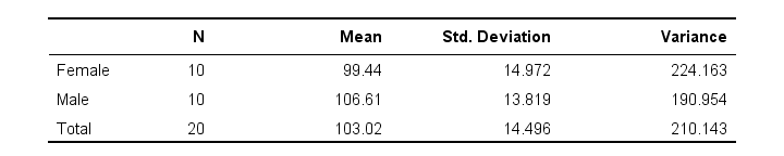
These sample means differ by some (99 - 106 =) -7 minutes: on average, females spend some 7 minutes less on the phone than males. But that's just our tiny samples. What can we say about the entire populations? We'll find out by starting off with the null hypothesis.

Null Hypothesis

The null hypothesis for an independent samples t-test is (usually) that the 2 population means are equal. If this is really true, then we may easily find slightly different means in our samples. So precisely what difference can we expect? An intuitive way for finding out is a simple simulation.

Simulation

I created a fake dataset containing the entire populations of 1,000 males and 1,000 females. On average, both groups spend 103 minutes on the phone with a standard-deviation of 14.5. Note that the null hypothesis of equal means is clearly true for these populations.
I then sampled 10 males and 10 females and computed the mean difference. And then I repeated that process 999 times, resulting in the 1,000 sample mean differences shown below.

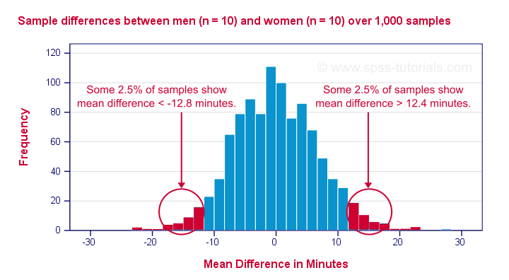
First off, the mean differences are roughly normally distributed. Most of the differences are close to zero -not surprising because the population difference is zero. But what's really interesting is that mean differences between, say, -12.5 and 12.5 are pretty common and make up 95% of my 1,000 outcomes. This suggests that an absolute difference of 12.5 minutes is needed for statistical significance at α = 0.05.
Last, the standard deviation of our 1,000 mean differences -the standard error- is 6.4. Note that some 95% of all outcomes lie between -2 and +2 standard errors of our (zero) mean. This is one of the best known rules of thumb regarding the normal distribution.
Now, an easier -though less visual- way to draw these conclusions is using a couple of simple formulas.

Test Statistic

Again: what is a “normal” sample mean difference if the population difference is zero? First off, this depends on the population standard deviation of our outcome variable. We don't usually know it but we can estimate it with $$Sw = \sqrt{\frac{(n_1 - 1)\;S^2_1 + (n_2 - 1)\;S^2_2}{n_1 + n_2 - 2}}$$
in which \(Sw\) denotes our estimated population standard deviation. For our data, this boils down to $$Sw = \sqrt{\frac{(10 - 1)\;224 + (10 - 1)\;191}{10 + 10 - 2}} ≈ 14.4$$
Second, our mean difference should fluctuate less -that is, have a smaller standard error- insofar as our sample sizes are larger. The standard error is calculated as $$Se = Sw\sqrt{\frac{1}{n_1} + \frac{1}{n_2}}$$
and this gives us $$Se = 14.4\; \sqrt{\frac{1}{10} + \frac{1}{10}} ≈ 6.4$$
If the population mean difference is zero, then -on average- the sample mean difference will be zero as well. However, it will have a standard deviation of 6.4. We can now just compute a z-score for the sample mean difference but -for some reason- it's called T instead of Z: $$T = \frac{\overline{X}_1 - \overline{X}_2}{Se}$$
which, for our data, results in $$T = \frac{99.4 - 106.6}{6.4} ≈ -1.11$$
Right, now this is our test statistic: a number that summarizes our sample outcome with regard to the null hypothesis. T is basically the standardized sample mean difference; T = -1.11 means that our difference of -7 minutes is roughly 1 standard deviation below the average of zero.

Assumptions

Our t-value follows a t distribution but only if the following assumptions are met:

1. Independent observations or, precisely, independent and identically distributed variables.
2. Normality: the outcome variable follows a normal distribution in the population. This assumption is not needed for reasonable sample sizes (say, N > 25).
3. Homogeneity: the outcome variable has equal standard deviations in our 2 (sub)populations. This is not needed if the sample sizes are roughly equal. Levene's test is sometimes used for testing this assumption.

If our data meet these assumptions, then T follows a t-distribution with (n1 + n2 -2) degrees of freedom (df). In our example, df = (10 + 10 - 2) = 18. The figure below shows the exact distribution. Note that we need an absolute t-value of 2.1 for 2-tailed significance at α = 0.05.

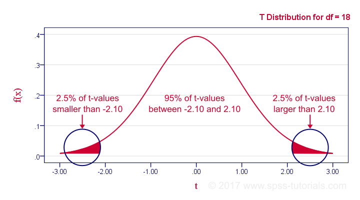
Minor note: as df becomes larger, the t-distribution approximates a standard normal distribution. The difference is hardly noticeable if df > 15 or so.

Statistical Significance

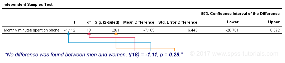
Last but not least, our mean difference of -7 minutes is not statistically significant: t(18) = -1.11, p ≈ 0.28. This means we've a 28% chance of finding our sample mean difference -or a more extreme one- if our population means are really equal; it's a normal outcome that doesn't contradict our null hypothesis.
Our final figure shows these results as obtained from SPSS.

Effect Size

Finally, the effect size measure that's usually preferred is Cohen’s D, defined as $$D = \frac{\overline{X}_1 - \overline{X}_2}{Sw}$$

in which \(Sw\) is the estimated population standard deviation we encountered earlier. That is, Cohen’s D is the number of standard deviations between the 2 sample means. So what is a small or large effect? The following rules of thumb have been proposed:

• D = 0.20 indicates a small effect;
• D = 0.50 indicates a medium effect;
• D = 0.80 indicates a large effect.

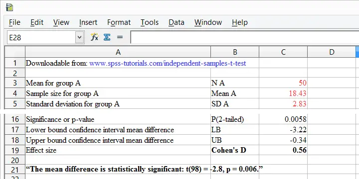
Cohen’s D is painfully absent from SPSS except for SPSS 27. However, you can easily obtain it from Cohens-d.xlsx. Just fill in 2 sample sizes, means and standard deviations and its formulas will compute everything you need to know.

Thanks for reading!

SPSS Independent Samples T-Test

A newly updated, ad-free video version of this tutorial
is included in our SPSS beginners course.

• Assumptions
• Independent Samples T-Test Flowchart
• Independent Samples T-Test Dialogs
• Output I - Significance Levels
• Output II - Effect Size
• APA Reporting - Tables & Text

Introduction & Example Data

An independent samples t-test examines if 2 populations
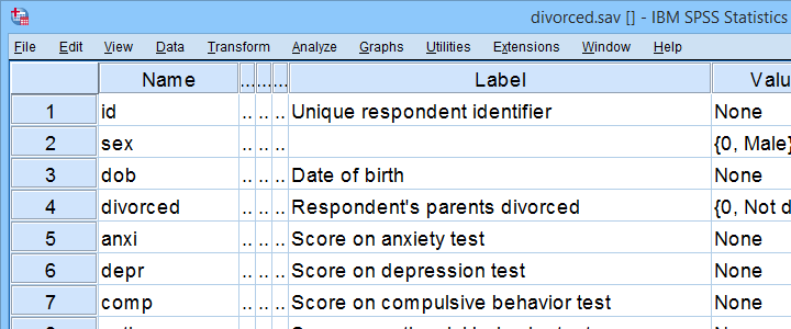
have equal means on some quantitative variable. For instance, do children from divorced versus non-divorced parents have equal mean scores on psychological tests? We'll walk you through using divorced.sav, part of which is shown below.

First off, I'd like to shorten some variable labels with the syntax below. Doing so prevents my tables from becoming too wide to fit the pages in my final thesis.

Let's now take a quick look at what's in our data in the first place. Does everything look plausible? Are there any outliers or missing values? I like to find out by running some quick histograms from the syntax below.

Result

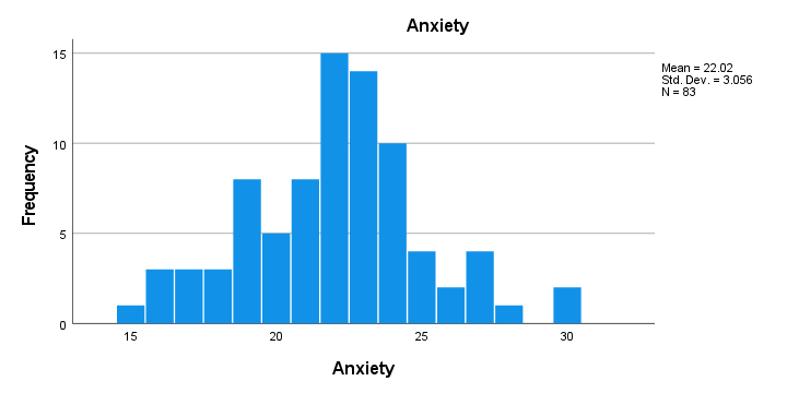
• First, note that all frequency distributions look plausible: we don't see anything weird or unusual.
• Also, none of our histograms show any clear outliers on any of our variables.
• Finally, note that N = 83 for each variable. Since this is our total sample size, this implies that none of them contain any missing values.

After this quick inspection, I like to create a table with sample sizes, means & standard deviations of all dependent variables for both groups separately.

The best way to do so is from Analyze Compare Means Means but the syntax is so simple that just typing it is faster:

Result

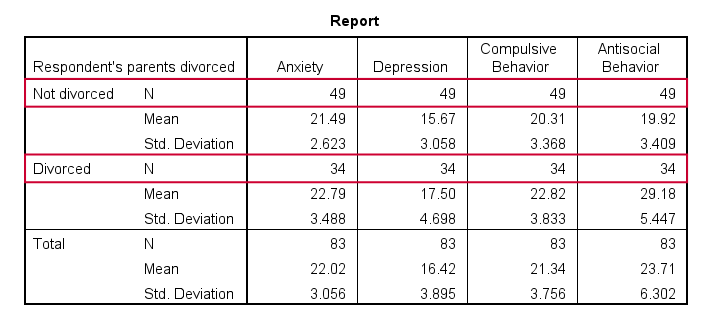
• Note that n = 49 (parents not divorced) and n = 34 (parents divorced) for all dependent variables.
• Also note that children from divorced parents have slightly higher mean scores on most tests. The difference on antisocial behavior (final column) is especially large.

Now, the big question is: can we conclude from these sample differences
that the entire populations are also different? An independent samples t-test will answer precisely that. It does, however, require some assumptions.

Assumptions

• independent observations. This often holds if each row of data represents a different person.
• Normality: the dependent variable must follow a normal distribution in each subpopulation. This is not needed if both n ≥ 25 or so.
• Homogeneity of variances: both subpopulations must have equal variances on the dependent variable. This is not needed if both sample sizes are roughly equal.

If sample sizes are not roughly equal, then Levene's test may be used to test if homogeneity is met. If that's not the case, then you should report adjusted results. These are shown in the SPSS t-test output under “equal variances not assumed”.

More generally, this procedure is known as the Welch test and also applies to ANOVA as covered in SPSS ANOVA - Levene’s Test “Significant”.

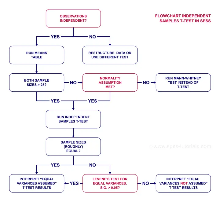
Now, if that's a little too much information, just try and follow the flowchart below.

Independent Samples T-Test Flowchart

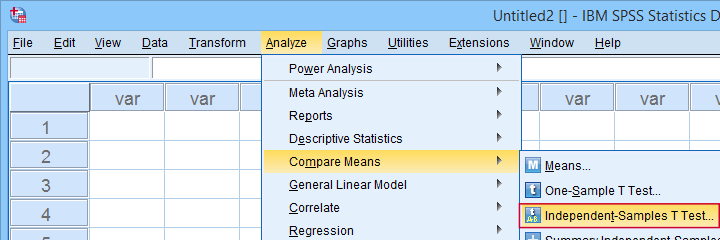
Independent Samples T-Test Dialogs

First off, let's navigate to Analyze Compare Means Independent Samples T Test as shown below.

Next, we fill out the dialog as shown below.

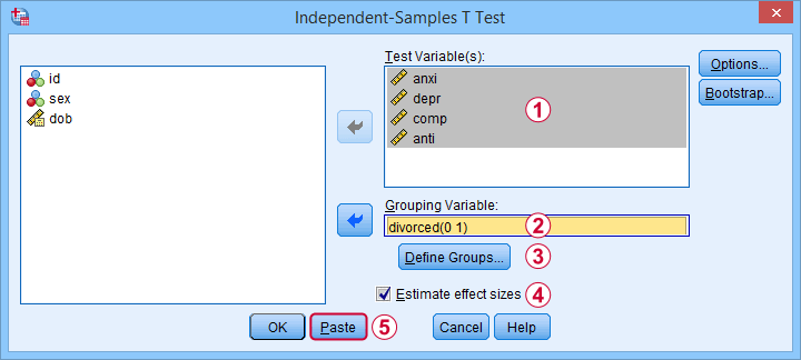
Sadly, the effect sizes are only available in SPSS version 27 and higher. Since they're very useful, try and upgrade if you're still on SPSS 26 or older.

Anyway, completing these steps results in the syntax below. Let's run it.

Output I - Significance Levels

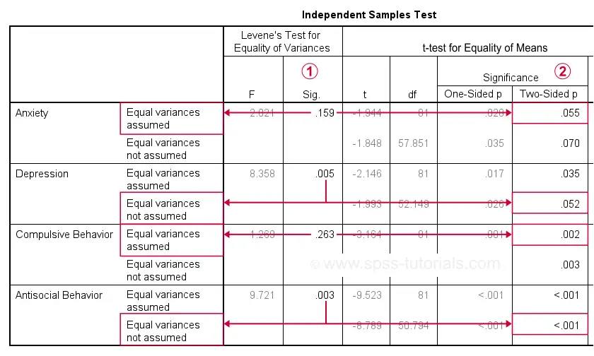
As previously discussed, each dependent variable has 2 lines of results. Which line to report depends on Levene’s test because our sample sizes are not (roughly) equal:

• if Levene’s test “Sig” or p ≥ .05, then report the “Equal variances assumed” t-test results.
• otherwise, report the “Equal variances not assumed” t-test results.

Following this procedure, we conclude that the mean differences on anxiety (p = .055) and depression (p = .052) are not statistically significant.

The differences on compulsive behavior (p = .002) and antisocial behavior (p < .001), however are both highly “significant”.

This last finding means that our sample differences are highly unlikely if our populations have exactly equal means. The output also includes the mean differences and their confidence intervals.

For example, the mean difference on anxiety is -1.30 points on the anxiety test. But what we don't know, is: should we consider this a small, medium or large difference? We'll answer just that by standardizing our mean differences into effect size measures.

Output II - Effect Size

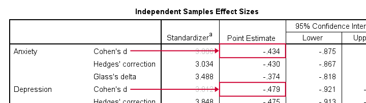
The most common effect size measure for t-tests is Cohen’s D, which we find under “point estimate” in the effect sizes table (only available for SPSS version 27 onwards).

Some general rules of thumb are that

• |d| = 0.20 indicates a small effect;
• |d| = 0.50 indicates a medium effect;
• |d| = 0.80 indicates a large effect.

Like so, we could consider d = -0.43 for our anxiety test roughly a medium effect of divorce and so on.

APA Reporting - Tables & Text

The figure below shows the exact APA style table for reporting the results obtained during this tutorial.

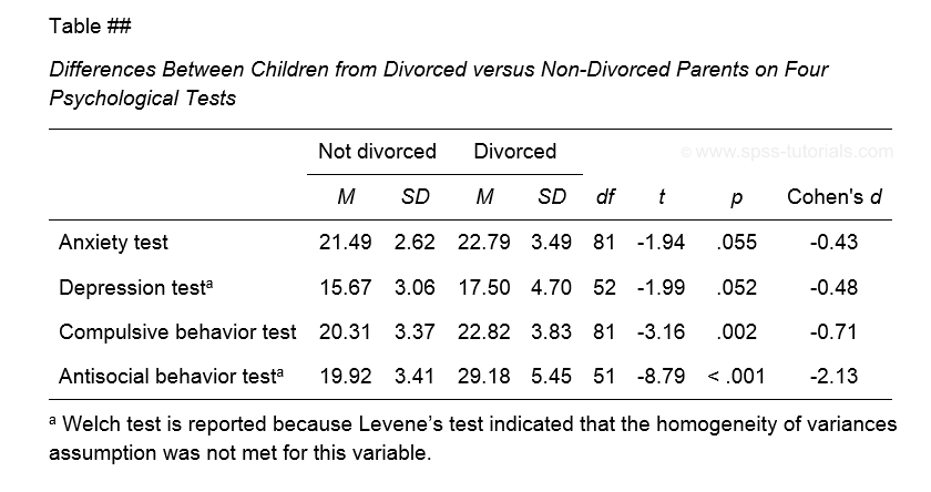
Minor note: if all tests have equal df (degrees of freedom), you may omit this column. In this case, add df to the column header for t as in t(81).

This table was created by combining results from 3 different SPSS output tables in Excel. This doesn't have to be a lot of work if you master a couple of tricks. I hope to cover these in a separate tutorial some time soon.

If you prefer reporting results in text format, follow the example below.

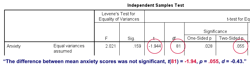
Note that d = -0.43 refers to Cohen’s D here, which is obtained from a separate table as previously discussed.

Final Notes

Most textbooks will tell you to

• use an independent samples t-test for comparing means between 2 subpopulations and
• use ANOVA for comparing means among 3+ subpopulations.

So what happens if we run ANOVA instead of t-tests on the 2 groups in our data? The syntax below does just that.

Those who ran this syntax will quickly see that most results are identical. This is because an independent samples t-test is a special case of ANOVA. There's 2 important differences, though:

• ANOVA comes up with a single p-value which is identical to p(2-tailed) from the corresponding t-test;
• the effect size for ANOVA is (partial) eta squared rather than Cohen’s D.

This raises an important question: why do we report different measures for comparing
2 rather than 3+ groups? My answer: we shouldn't. And this implies that we should

• always report p(2-tailed) for t-tests, never p(1-tailed);
• report eta-squared as the effect size for t-tests and abandon Cohen’s D.

Thanks for reading!