SPSS ANCOVA – Beginners Tutorial
- ANCOVA - Null Hypothesis
- ANCOVA Assumptions
- SPSS ANCOVA Dialogs
- SPSS ANCOVA Output - Between-Subjects Effects
- SPSS ANCOVA Output - Adjusted Means
- ANCOVA - APA Style Reporting
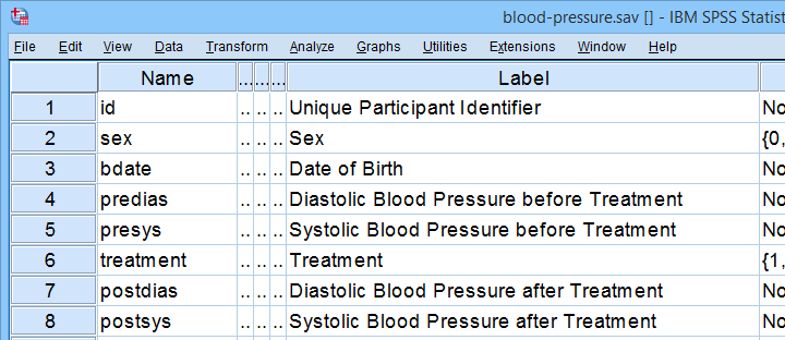
A pharmaceutical company develops a new medicine against high blood pressure. They tested their medicine against an old medicine, a placebo and a control group. The data -partly shown below- are in blood-pressure.sav.
Our company wants to know if their medicine outperforms the other treatments: do these participants have lower blood pressures than the others after taking the new medicine? Since treatment is a nominal variable, this could be answered with a simple ANOVA.
Now, posttreatment blood pressure is known to correlate strongly with pretreatment blood pressure. This variable should therefore be taken into account as well. The relation between pretreatment and posttreatment blood pressure could be examined with simple linear regression because both variables are quantitative.
We'd now like to examine the effect of medicine while controlling for pretreatment blood pressure. We can do so by adding our pretest as a covariate to our ANOVA. This now becomes ANCOVA -short for analysis of covariance. This analysis basically combines ANOVA with regression.
Surprisingly, analysis of covariance does not actually involve covariances as discussed in Covariance - Quick Introduction.
ANCOVA - Null Hypothesis
Generally, ANCOVA tries to demonstrate some effect by rejecting the null hypothesis that all population means are equal when controlling for 1+ covariates. For our example, this translates to “average posttreatment blood pressures are equal for all treatments when controlling for pretreatment blood pressure”. The basic analysis is pretty straightforward but it does require quite a few assumptions. Let's look into those first.
ANCOVA Assumptions
- independent observations;
- normality: the dependent variable must be normally distributed within each subpopulation. This is only needed for small samples of n < 20 or so;
- homogeneity: the variance of the dependent variable must be equal over all subpopulations. This is only needed for sharply unequal sample sizes;
- homogeneity of regression slopes: the b-coefficient(s) for the covariate(s) must be equal among all subpopulations.
- linearity: the relation between the covariate(s) and the dependent variable must be linear.
Taking these into account, a good strategy for our entire analysis is to
- first run some basic data checks: histograms and descriptive statistics give quick insights into frequency distributions and sample sizes. This tells us if we even need assumptions 2 and 3 in the first place.
- see if assumptions 4 and 5 hold by running regression analyses for our treatment groups separately;
- run the actual ANCOVA and see if assumption 3 -if necessary- holds.
Data Checks I - Histograms
Let's first see if our blood pressure variables are even plausible in the first place. We'll inspect their histograms by running the syntax below. If you prefer to use SPSS’ menu, consult Creating Histograms in SPSS.
frequencies predias postdias
/format notable
/histogram.
Result
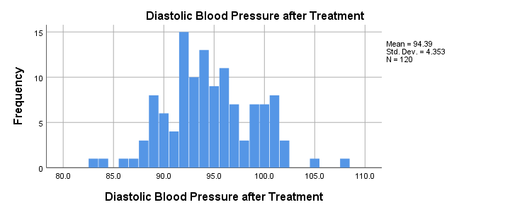
Conclusion: the frequency distributions for our blood pressure measurements look plausible: we don't see any very low or high values. Neither shows a lot of skewness or kurtosis and they both look reasonably normally distributed.
Data Checks II - Descriptive Statistics
Next, let's look into some descriptive statistics, especially sample sizes. We'll create and inspect a table with the
- sample sizes,
- means and
- standard deviations
of the outcome variable and the covariate for our treatment groups separately. We could do so from
![]()
![]() or -faster- straight from syntax.
or -faster- straight from syntax.
means predias postdias by treatment
/statistics anova.
Result
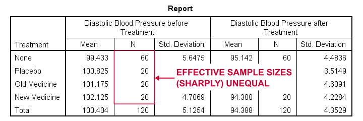
The main conclusions from our output are that
- all treatment groups have reasonable samples sizes of at least n = 20. This means we don't need to bother about the normality assumption. Otherwise, we could use a Shapiro-Wilk normality test or a Kolmogorov-Smirnov test but we rather avoid these.
- the treatment groups have sharply unequal sample sizes. This implies that our ANCOVA will need to satisfy the homogeneity of variance assumption.
- the ANOVA results (not shown here) tell us that the posttreatment means don't differ statistically significantly, F(3,116) = 1.619, p = 0.189. However, this test did not yet include our covariate -pretreatment blood pressure.
So much for our basic data checks. We'll now look into the regression results and then move on to the actual ANCOVA.
Separate Regression Lines for Treatment Groups
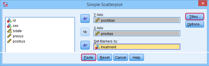
Let's now see if our regression slopes are equal among groups -one of the ANCOVA assumptions. We'll first just visualize them in a scatterplot as shown below.
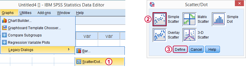
Clicking results in the syntax below.
GRAPH
/SCATTERPLOT(BIVAR)=predias WITH postdias BY treatment
/MISSING=LISTWISE.GRAPH
/TITLE='Diastolic Blood Pressure by Treatment'.
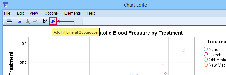
*Double-click resulting chart and click "Add fit line at subgroups" icon.
SPSS now creates a scatterplot with different colors for different treatment groups. Double-clicking it opens it in a Chart Editor window. Here we click the “Add Fit Lines at Subgroups” icon as shown below.
Result
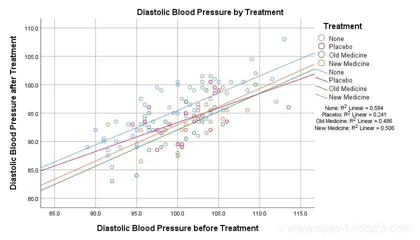
The main conclusion from this chart is that the regression lines are almost perfectly parallel: our data seem to meet the homogeneity of regression slopes assumption required by ANCOVA.
Furthermore, we don't see any deviations from linearity: this ANCOVA assumption also seems to be met. For a more thorough linearity check, we could run the actual regressions with residual plots. We did just that in SPSS Moderation Regression Tutorial.
Now that we checked some assumptions, we'll run the actual ANCOVA twice:
- the first run only examines the homogeneity of regression slopes assumption. If this holds, then there should not be any covariate by treatment interaction-effect.
- the second run tests our null hypothesis: are all population means equal when controlling for our covariate?
SPSS ANCOVA Dialogs
Let's first navigate to
![]()
![]() and fill out the dialog boxes as shown below.
and fill out the dialog boxes as shown below.
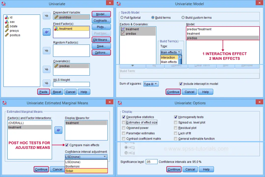
Clicking generates the syntax shown below.
UNIANOVA postdias BY treatment WITH predias
/METHOD=SSTYPE(3)
/INTERCEPT=INCLUDE
/EMMEANS=TABLES(treatment) WITH(predias=MEAN) COMPARE ADJ(SIDAK)
/PRINT ETASQ HOMOGENEITY
/CRITERIA=ALPHA(.05)
/DESIGN=predias treatment predias*treatment. /* predias*treatment adds interaction effect to model.
Result
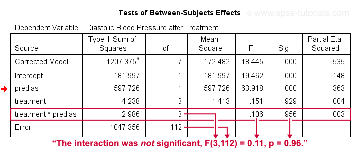
First note that our covariate by treatment interaction is not statistically significant at all: F(3,112) = 0.11, p = 0.96. This means that the regression slopes for the covariate don't differ between treatments: the homogeneity of regression slopes assumption seems to hold almost perfectly.
For these data, this doesn't come as a surprise: we already saw that the regression lines for different treatment groups were roughly parallel. Our first ANCOVA is basically a more formal way to make the same point.
SPSS ANCOVA II - Main Effects
We now run simply rerun our ANCOVA as previously. This time, however, we'll remove the covariate by treatment interaction effect. Doing so results in the syntax shown below.
UNIANOVA postdias BY treatment WITH predias
/METHOD=SSTYPE(3)
/INTERCEPT=INCLUDE
/EMMEANS=TABLES(treatment) WITH(predias=MEAN) COMPARE ADJ(SIDAK)
/PRINT ETASQ HOMOGENEITY
/CRITERIA=ALPHA(.05)
/DESIGN=predias treatment. /* only test for 2 main effects.
SPSS ANCOVA Output I - Levene's Test
Since our treatment groups have sharply unequal sample sizes, our data need to satisfy the homogeneity of variance assumption. This is why we included Levene's test in our analysis. Its results are shown below.
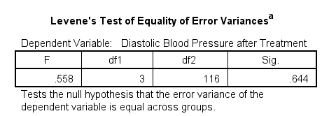
Conclusion: we don't reject the null hypothesis of equal error variances, F(3,116) = 0.56, p = 0.64. Our data meets the homogeneity of variances assumption. This means we can confidently report the other results.
SPSS ANCOVA Output - Between-Subjects Effects
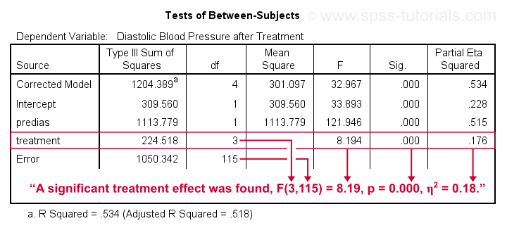
Conclusion: we reject the null hypothesis that our treatments result in equal mean blood pressures, F(3,115) = 8.19, p = 0.000.
Importantly, the effect size for treatment is between medium and large: partial eta squared (written as η2) = 0.176.
Apparently, some treatments perform better than others after all. Interestingly, this treatment effect was not statistically significant before including our pretest as a covariate.
So which treatments perform better or worse? For answering this, we first inspect our estimated marginal means table.
SPSS ANCOVA Output - Adjusted Means
One role of covariates is to adjust posttest means for any differences among the corresponding pretest means. These adjusted means and their standard errors are found in the Estimated Marginal Means table shown below.
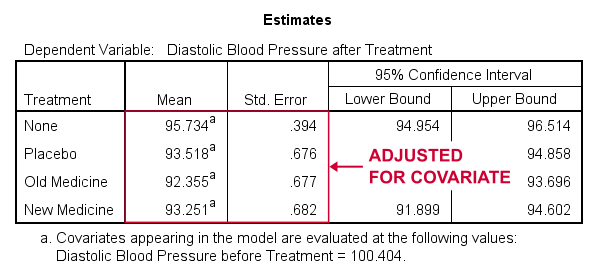
These adjusted means suggest that all treatments result in lower mean blood pressures than “None”. The lowest mean blood pressure is observed for the old medicine. So precisely which mean differences are statistically significant? This is answered by post hoc tests which are found in the Pairwise Comparisons table (not shown here). This table shows that all 3 treatments differ from the control group but none of the other differences are statistically significant. For a more detailed discussion of post hoc tests, see SPSS - One Way ANOVA with Post Hoc Tests Example.
ANCOVA - APA Style Reporting
For reporting our ANCOVA, we'll first present descriptive statistics for
- our covariate;
- our dependent variable (unadjusted);
- our dependent variable (adjusted for the covariate).
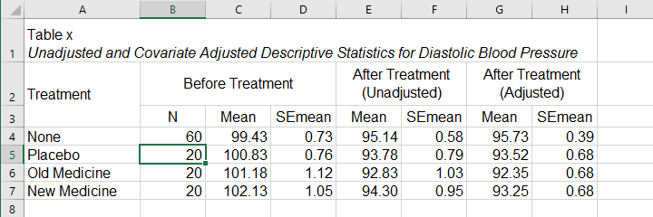
What's interesting about this table is that the posttest means are hardly adjusted by including our covariate. However, the covariate greatly reduces the standard errors for these means. This is why the mean differences are statistically significant only when the covariate is included. The adjusted descriptives are obtained from the final ANCOVA results. The unadjusted descriptives can be created from the syntax below.
means predias postdias by treatment
/cells count mean semean.
The exact APA table is best created by copy-pasting these statistics into Excel or Googlesheets.
Second, we'll present a standard ANOVA table for the effects included in our final model and error.
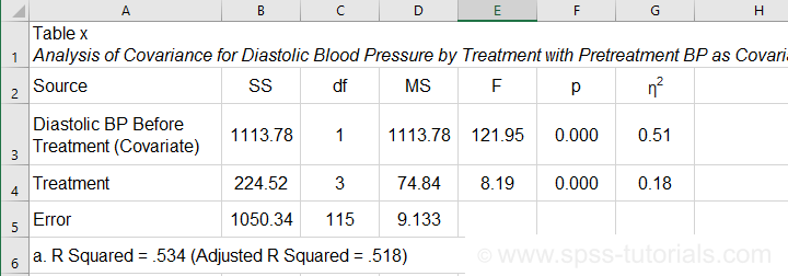
This table is constructed by copy-pasting the SPSS output table into Excel and removing the redundant rows.
Final Notes
So that'll do for a very solid but simple ANCOVA in SPSS. We could have written way more about this example analysis as there's much -much- more to say about the output. We'd also like to cover the basic ideas behind ANCOVA into more detail but that really requires a separate tutorial which we hope to write in some weeks from now.
Hope my tutorial has been helpful anyway. So last off:
thanks for reading!
Repeated Measures ANOVA – Simple Introduction
Null Hypothesis
The null hypothesis for a repeated measures ANOVA is that 3(+) metric variables have identical means in some population.
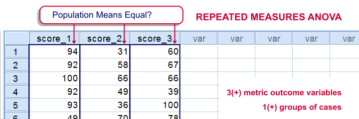
The variables are measured on the same subjects so we're looking for within-subjects effects (differences among means). This basic idea is also referred to as dependent, paired or related samples in -for example- nonparametric tests.
But anyway: if all population means are really equal, we'll probably find slightly different means in a sample from this population. However, very different sample means are unlikely in this case. These would suggest that the population means weren't equal after all.
Repeated measures ANOVA basically tells us how likely our sample mean differences are if all means are equal in the entire population.
Repeated Measures ANOVA - Assumptions
- Independent observations or, precisely, Independent and identically distributed variables;
- Normality: the test variables follow a multivariate normal distribution in the population;
- Sphericity: the variances of all difference scores among the test variables must be equal in the population. Sphericity is sometimes tested with Mauchly’s test. If sphericity is rejected, results may be corrected with the Huynh-Feldt or Greenhouse-Geisser correction.
Repeated Measures ANOVA - Basic Idea
We'll show some example calculations in a minute. But first: how does repeated measures ANOVA basically work? First off, our outcome variables vary between and within our subjects. That is, differences between and within subjects add up to a total amount of variation among scores. This amount of variation is denoted as SStotal where SS is short for “sums of squares”.
We'll then split our total variance into components and inspect which component accounts for how much variance as outlined below. Note that “df” means “degrees of freedom”, which we'll get to later.
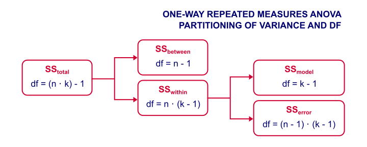
Now, we're not interested in how the scores differ between subjects. We therefore remove this variance from the total variance and ignore it. We're then left with just SSwithin (variation within subjects).
The variation within subjects may be partly due to our variables having different means. These different means make up our model. SSmodel is the amount of variation it accounts for.
Next, our model doesn't usually account for all of the variation between scores within our subjects. SSerror is the amount of variance that our model does not account for.
Finally, we compare two sources of variance: if SSmodel is large and SSerror is small, then variation within subjects is mostly due to our model (consisting of different variable means). This results in a large F-value, which is unlikely if the population means are really equal. In this case, we'll reject the null hypothesis and conclude that the population means aren't equal after all.
Repeated Measures ANOVA - Basic Formulas
We'll use the following notation in our formulas:
- \(n\) denotes the number of subjects;
- \(k\) denotes the number of variables;
- \(Xij\) denotes the score of subject \(i\) on variable \(j\);
- \(Xi.\) denotes the mean for subject \(i\);
- \(X.j\) denotes the mean of variable \(j\);
- \(X..\) denotes the grand mean.
Now, the formulas for the sums of squares, degrees of freedom and mean squares are
$$SS_{within} = \sum_{i=1}^n\sum_{j=1}^k(Xij - Xi.)^2$$
$$SS_{model} = n \sum_{j=1}^k(X.j - X..)^2$$
$$SS_{error} = SS_{within} - SS_{model}$$
$$df_{model} = k - 1$$
$$df_{error} = (k - 1)\cdot(n - 1)$$
$$MS_{model} = \frac{SS_{model}}{df_{model}}$$
$$MS_{error} = \frac{SS_{error}}{df_{error}}$$
$$F = \frac{MS_{model}}{MS_{error}}$$
Repeated Measures ANOVA - Example
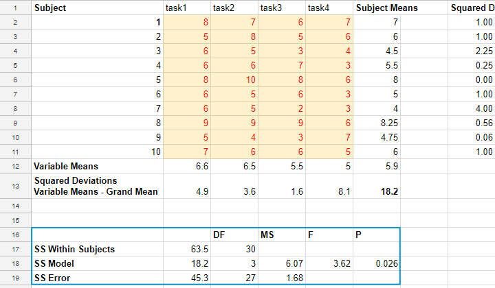
We had 10 people perform 4 memory tasks. The data thus collected are listed in the table below. We'd like to know if the population mean scores for all four tasks are equal.
| Subject | task1 | task2 | task3 | task4 | Subject Mean |
|---|---|---|---|---|---|
| 1 | 8 | 7 | 6 | 7 | 7 |
| 2 | 5 | 8 | 5 | 6 | 6 |
| 3 | 6 | 5 | 3 | 4 | 4.5 |
| 4 | 6 | 6 | 7 | 3 | 5.5 |
| 5 | 8 | 10 | 8 | 6 | 8 |
| 6 | 6 | 5 | 6 | 3 | 5 |
| 7 | 6 | 5 | 2 | 3 | 4 |
| 8 | 9 | 9 | 9 | 6 | 8.25 |
| 9 | 5 | 4 | 3 | 7 | 4.75 |
| 10 | 7 | 6 | 6 | 5 | 6 |
| Variable Mean | 6.6 | 6.5 | 5.5 | 5 | 5.9 (grand mean) |
If we apply our formulas to our example data, we'll get
$$SS_{within} = (8 - 7)^2 + (7 - 7)^2 + ... + (5 - 6)^2 = 63.5$$
$$SS_{model} = 10 \cdot((6.6 - 5.9)^2 + (6.5 - 5.9)^2 + (5.5 - 5.9)^2 + (5 - 5.9)^2) = 18.2$$
$$SS_{error} = 63.5 - 18.2 = 45.3$$
$$MS_{model} = \frac{18.2}{3} = 6.07$$
$$MS_{error} = \frac{45.3}{27} = 1.68$$
$$F = \frac{6.07}{1.68} = 3.62$$
$$P(F(3,27) > 3.62) \approx 0.026$$
The null hypothesis is usually rejected when p < 0.05. Conclusion: the population means probably weren't equal after all.
Repeated Measures ANOVA - Software
We computed the entire example in the Googlesheet shown below. It's accessible to all readers so feel free to take a look at the formulas we use.
Although you can run the test in a Googlesheet, you probably want to use decent software for running a repeated measures ANOVA. It's not included in SPSS by default unless you have the advanced statistics option installed. An outstanding example of repeated measures ANOVA in SPSS is SPSS Repeated Measures ANOVA.
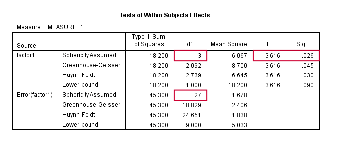
The figure below shows the SPSS output for the example we ran in this tutorial.
Factorial Repeated Measures ANOVA
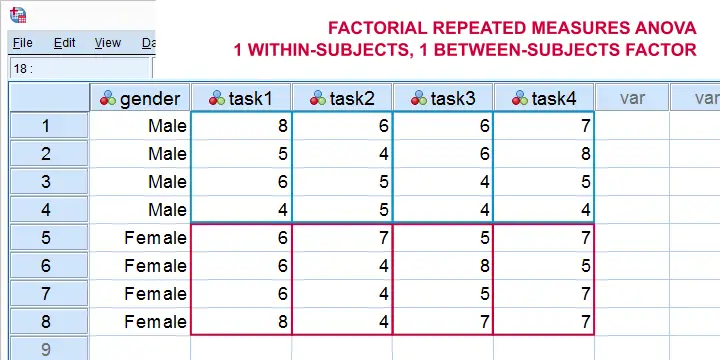
Thus far, our discussion was limited to one-way repeated measures ANOVA with a single within-subjects factor. We can easily extend this to a factorial repeated measures ANOVA with one within-subjects and one between-subjects factor. The basic idea is shown below. For a nice example in SPSS, see SPSS Repeated Measures ANOVA - Example 2.
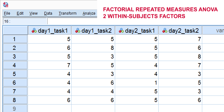
Alternatively, we can extend our model to a factorial repeated measures ANOVA with 2 within-subjects factors. The figure below illustrates the basic idea.
Finally, we could further extend our model into a 3(+) way repeated measures ANOVA. (We speak of “repeated measures ANOVA” if our model contains at least 1 within-subjects factor.)
Right, so that's about it I guess. I hope this tutorial has clarified some basics of repeated measures ANOVA.
Thanks for reading!
ANOVA – Super Simple Introduction
- ANOVA - Null Hypothesis
- Test Statistic - F
- Assumptions for ANOVA
- Effect Size - (Partial) Eta Squared
- ANOVA - Post Hoc Tests
ANOVA -short for “analysis of variance”- is a statistical technique
for testing if 3(+) population means are all equal.
The two simplest scenarios are
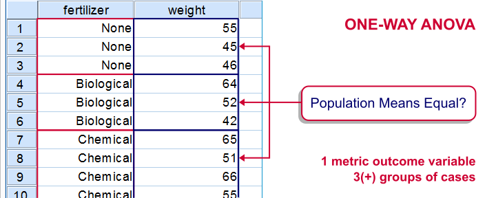
- one-way ANOVA for comparing 3(+) groups on 1 variable: do all children from school A, B and C have equal mean IQ scores? For 2 groups, one-way ANOVA is identical to an independent samples t-test.
- repeated measures ANOVA for comparing 3(+) variables in 1 group: is the mean rating for beer A, B and C equal for all people?For 2 variables, repeated measures ANOVA is identical to a paired samples t-test.
The figure below visualizes the basic question for one-way ANOVA.
Simple Example - One-Way ANOVA
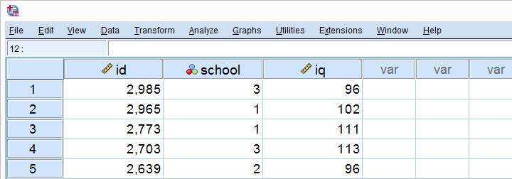
A scientist wants to know if all children from schools A, B and C have equal mean IQ scores. Each school has 1,000 children. It takes too much time and money to test all 3,000 children. So a simple random sample of n = 10 children from each school is tested.
Part of these data -available from this Googlesheet are shown below.
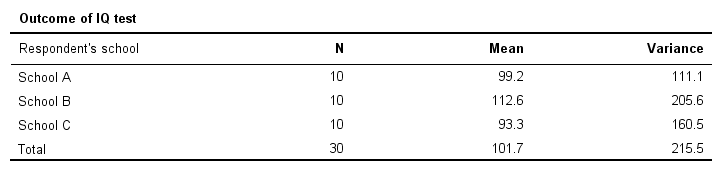
Descriptives Table
Right, so our data contain 3 samples of 10 children each with their IQ scores. Running a simple descriptives table immediately tells us the mean IQ scores for these samples. The result is shown below.
For making things clearer, let's visualize the mean IQ scores per school in a simple bar chart.
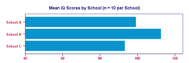
Clearly, our sample from school B has the highest mean IQ - roughly 113 points. The lowest mean IQ -some 93 points- is seen for school C.
Now, here's the problem: our mean IQ scores are only based on tiny samples of 10 children per school. So couldn't it be that
all 1,000 children per school have the same mean IQ?
Perhaps we just happened to sample the smartest children from school B and the dumbest children from school C?“Dumbest” isn't really appropriate here: these children may have terrific talents that -unfortunately for them- aren't measured by the test administered. However, a discussion of the usefulness of IQ tests is beyond the scope of this tutorial. Is that realistic? We'll try and show that this statement -our null hypothesis- is not credible given our data.
ANOVA - Null Hypothesis
The null hypothesis for (any) ANOVA is that all population means are exactly equal. If this holds, then our sample means will probably differ a bit. After all, samples always differ a bit from the populations they represent. However, the sample means probably shouldn't differ too much. Such an outcome would be unlikely under our null hypothesis of equal population means. So if we do find this, we'll probably no longer believe that our population means were really equal.
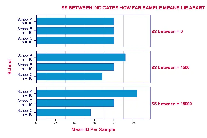
ANOVA - Sums of Squares Between
So precisely how different are our 3 sample means? How far do these numbers lie apart? A number that tells us just that is the variance. So we'll basically compute the variance among our 3 sample means.
As you may (or may not) understand from the ANOVA formulas, this starts with the sum of the squared deviations between the 3 sample means and the overall mean. The outcome is known as the “sums of squares between” or SSbetween. So
sums of squares between expresses
the total amount of dispersion among the sample means.
Everything else equal, larger SSbetween indicates that the sample means differ more. And the more different our sample means, the more likely that our population means differ as well.
Degrees of Freedom and Mean Squares Between
When calculating a “normal” variance, we divide our sums of squares by its degrees of freedom (df). When comparing k means, the degrees of freedom (df) is (k - 1).
Dividing SSbetween by (k - 1) results in mean squares between: MSbetween. In short,
mean squares between
is basically the variance among sample means.
MSbetween thus indicates how far our sample means differ (or lie apart). The larger this variance between means, the more likely that our population means differ as well.
ANOVA - Sums of Squares Within
If our population means are really equal, then what difference between sample means -MSbetween- can we reasonably expect? Well, this depends on the variance within subpopulations. The figure below illustrates this for 3 scenarios.
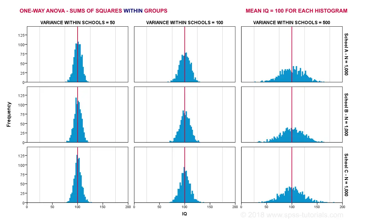
The 3 leftmost histograms show population distributions for IQ in schools A, B and C. Their narrowness indicates a small variance within each school. If we'd sample n = 10 students from each school,
should we expect very different sample means?
Probably not. Why? Well, due to the small variance within each school, the sample means will be close to the (equal) population means. These narrow histograms don't leave a lot of room for their sample means to fluctuate and -hence- differ.
The 3 rightmost histograms show the opposite scenario: the histograms are wide, indicating a large variance within each school. If we'd sample n = 10 students from each school, the means in these samples may easily differ quite a lot. In short,
larger variances within schools probably result in a
larger variance between sample means per school.
We basically estimate the within-groups population variances from the within-groups sample variances. Makes sense, right? The exact calculations are in the ANOVA formulas and this Googlesheet. In short:
- sums of squares within (SSwithin) indicates the total amount of dispersion within groups;
- degrees of freedom within (DFwithin) is (n - k) for n observations and k groups and
- mean squares within (MSwithin) -basically the variance within groups- is SSwithin / DFwithin.
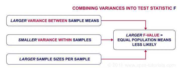
ANOVA Test Statistic - F
So how likely are the population means to be equal? This depends on 3 pieces of information from our samples:
- the variance between sample means (MSbetween);
- the variance within our samples (MSwithin) and
- the sample sizes.
We basically combine all this information into a single number: our test statistic F. The diagram below shows how each piece of evidence impacts F.
Now, F itself is not interesting at all. However, we can obtain the statistical significance from F if it follows an F-distribution. It will do just that if 3 assumptions are met.
ANOVA - Assumptions
The assumptions for ANOVA are
- independent observations;
- normality: the outcome variable must follow a normal distribution in each subpopulation. Normality is really only needed for small sample sizes, say n < 20 per group.
- homogeneity: the variances within all subpopulations must be equal. Homogeneity is only needed if sample sizes are very unequal. In this case, Levene's test indicates if it's met.
If these assumptions hold, then F follows an F-distribution with DFbetween and DFwithin degrees of freedom. In our example -3 groups of n = 10 each- that'll be F(2,27).
ANOVA - Statistical Significance
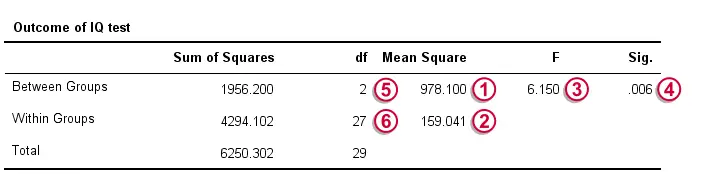
In our example, F(2,27) = 6.15. This huge F-value is strong evidence that our null hypothesis -all schools having equal mean IQ scores- is not true. If all assumptions are met, F follows the F-distribution shown below.
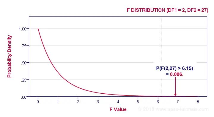
Given this distribution, we can look up that the statistical significance. We usually report: F(2,27) = 6.15, p = 0.006. If our schools have equal mean IQ's, there's only a 0.006 chance of finding our sample mean differences or larger ones. We usually say something is “statistically significant” if p < 0.05. Conclusion: our population means are very unlikely to be equal. The figure below shows how SPSS presents the output for this example.
Effect Size - (Partial) Eta Squared
So far, our conclusion is that the population means are not all exactly equal. Now, “not equal” doesn't say much. What I'd like to know is
exactly how different are the means?
A number that estimates just that is the effect size. An effect size measure for ANOVA is partial eta squared, written as η2.η is the Greek letter “eta”, pronounced as a somewhat prolonged “e”. For a one-way ANOVA, partial eta-squared is equal to simply eta-squared.
Technically,
(partial) eta-squared is the
proportion of variance accounted for by a factor.
Some rules of thumb are that
- η2 > 0.01 indicates a small effect;
- η2 > 0.06 indicates a medium effect;
- η2 > 0.14 indicates a large effect.
The exact calculation of eta-squared is shown in the formulas section. For now, suffice to say that η2 = 0.31 for our example. This huge -huge- effect size explains why our F-test is statistically significant despite our very tiny sample sizes of n = 10 per school.
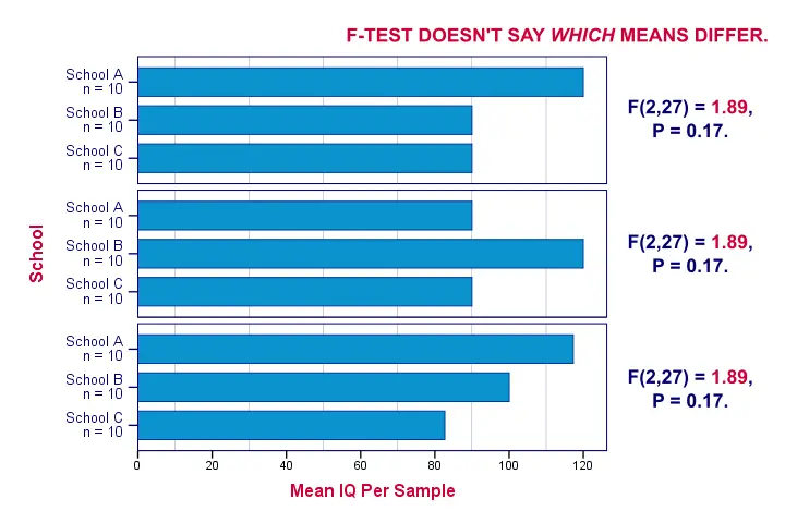
Post Hoc Tests - Tukey's HSD
So far, we concluded from our F-test that our population means are very unlikely to be (all) equal. The effect size, η2, told us that the difference is large. An unanswered question, though, is precisely which means are different? Different patterns of sample means may all result in the exact same F-value. The figure below illustrates this point with some possible scenarios.
One approach would be running independent samples t-tests on all possible pairs of means. For 3 means, that'll be A-B, A-C and B-C. However, as the number of means we compare grows, the number of all possible pairs rapidly increases.Precisely, k means result in 0.5 * k * (k - 1) distinct pairs. Like so, 3 means have 3 distinct pairs, 4 means have 6 distinct pairs and 5 means have 10 distinct pairs. And
each t-test has its own chance of drawing a wrong conclusion.
So the more t-tests we run, the bigger the risk of drawing at least one wrong conclusion.
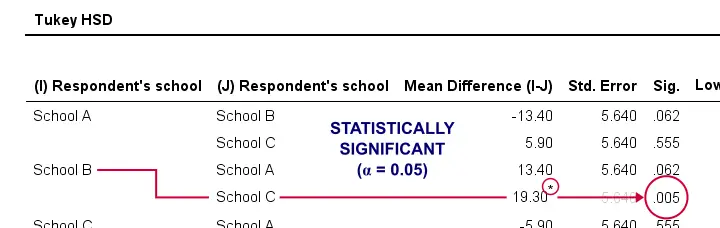
The most common solution to this problem is using Tukey's HSD (short for “Honestly Significant Difference”) procedure. You could think of it as running all possible t-tests for which the results have been corrected with some sort of Bonferroni correction but less conservative. The figure below shows some output from Tukey's HSD in SPSS.
Tukey's HSD is known as a post hoc test. “Post hoc” is Latin and literally means “after that”. This is because they are run only after the main F-test has indicated that not all means are equal. I don't entirely agree with this convention because
- post hoc tests may not indicate differences while the main F-test does;
- post hoc tests may indicate differences while the main F-test does not.
Say I'm comparing 5 means: A, B, C and D are equal but E is much larger than the others. In this case, the large difference between E and the other means will be strongly diluted when testing if all means are equal. So in this case
an overall F-test may not indicate any differences
while post hoc tests will.
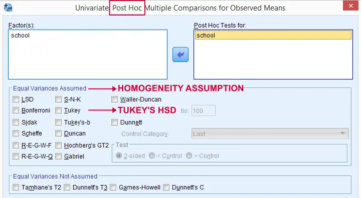
Last but not least, there's many other post hoc tests as well. Some require the homogeneity assumption and others don't. The figure below shows some examples.
ANOVA - Basic Formulas
For the sake of completeness, we'll list the main formulas used for the one-way ANOVA in our example. You can see them in action in this Googlesheet.
We'll start off with the between-groups variance:
$$SS_{between} = \Sigma\;n_j\;(\overline{X}_j - \overline{X})^2$$
where
- \(\overline{X}_j\) denotes a group mean;
- \(\overline{X}\) is the overall mean;
- \(n_j\) is the sample size per group.
For our example, this results in
$$SS_{between} = 10\;(99.2 - 101.7)^2 + 10\;(112.6 - 101.7)^2 + 10\;(93.3 - 101.7)^2 = 1956.2 $$
Next, for \(m\) groups,
$$df_{between} = m - 1$$
so \(df_{between}\) = 3 - 1 = 2 for our example data.
$$MS_{between} = \frac{SS_{between}}{df_{between}}$$
For our example, that'll be
$$\frac{1956.2}{2} = 978.1$$
We now turn to the within-groups variance. First off,
$$SS_{within} = \Sigma\;(X_i - \overline{X}_j)^2$$
where
- \(\overline{X}_j\) denotes a group mean;
- \(X_i\) denotes an individual observation (“data point”).
For our example, this'll be
$$SS_{within} = (90 - 99.2)^2 + (87 - 99.2)^2 + ... + (96 - 93.3)^2 = 4294.1$$
for \(n\) independent observations and \(m\) groups,
$$df_{within} = n - m$$
So for our example that'll be = 30 - 3 = 27.
$$MS_{within} = \frac{SS_{within}}{df_{within}}$$
For our example, this results in
$$\frac{4294.1}{27} = 159$$
We're now ready to calculate the F-statistic:
$$F = \frac{MS_{between}}{MS_{within}}$$
which results in
$$\frac{978.1}{159} = 6.15$$
Finally,
$$P = P(F(2,27) > 6.15) = 0.0063$$
Optionally, the effect size η2 is calculated as
$$Effect\;\;size\;\;\eta^2 = \frac{SS_{between}}{SS_{between} + SS_{within}}$$
For our example, that'll be
$$\frac{1956.2}{1956.2 + 4294.1} = 0.31$$
Thanks for reading.