Z-Test & Confidence Interval for Single Proportion

Z-Test and Confidence Interval Single Proportion

Z-Test Assumptions
Z-Test for Single Proportion - Formulas
Continuity Correction for Z-Test
Confidence Interval for Single Proportion
Agresti-Coull Adjustment for CI

A z-test for a single proportion examines if a
population proportion is likely to be x. Example: does a proportion of 0.60 (or 60%) of some population have antibodies against Covid-19?

If this is true, a sample proportion may differ somewhat from 0.60. However, a very different sample proportion suggests that our initial claim was wrong.

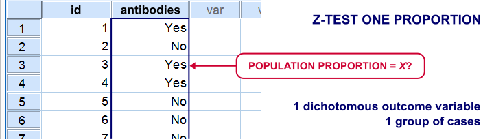
Note that this null hypothesis implies a dichotomous outcome variable: the only 2 possible outcomes are to carry or not to carry such antibodies.

Z-Test Single Proportion - Example

An epidemiologist believes that 60% of all Dutch adults carry antibodies against Covid-19;
she samples N = 112 people and administers PCR tests to them;
58 people (51.8%) out of 112 people test positive and thus carry antibodies.

Given this outcome, should she still believe that 60% of the entire population carry antibodies? A z-test answers just that but it does require some assumptions.

Z-Test Assumptions

A z-test for a single proportion requires two assumptions:

independent observations;
$n_1 \ge 15$ and $n_2 \ge 15$: our sample should contain at least some 15 observations for either possible outcome.

Standard textbooks^3,5 often propose $n_1 \ge 5$ and $n_2 \ge 5$ but recent studies suggest that these sample sizes are insufficient for accurate test results.²

Z-Test for Single Proportion - Formulas

If sample sizes are sufficient, a sample proportion is approximately normally distributed with

$$\mu_0 = \pi_0$$ and

$$\sigma_0 = SE_0 = \sqrt{\frac{\pi_0(1 - \pi_0)}{N}}$$

where

$\pi_0$ denotes the population proportion under the null hypothesis;
$SE_0$ denotes the standard error under the null hypothesis;
$N$ denotes the total sample size.

Our example examines if the population proportion $\pi_0$ is 0.60 using a total sample size of $N$ = 112 and therefore,

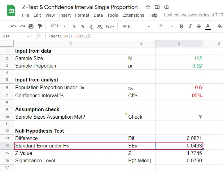
$$SE_0 = \sqrt{\frac{0.60(1 - 0.60)}{112}} = 0.046.$$

Using this outcome, we can standardize our sample proportion $pi$ into a z-score using

$$Z = \frac{pi - \pi_0}{SE_0}$$

Our sample came up with a proportion $pi$ of 0.52 because 58 out of 112 people carried Covid-19 antibodies. Therefore,

$$Z = \frac{0.52 - 0.60}{0.046} = -1.77$$

Finally,

$$p(2{\text -}tailed) = 2 \cdot p(z \lt -1.77) = 0.076.$$

This means that if the population proportion really is 0.60, there's a 0.076 (or 7.6%) probability of finding a sample proportion of 0.52 or a more extreme outcome in either direction. Conclusion: we do not reject the null hypothesis that $\pi_0 = 0.60$ if we test at the usual $\alpha$ = 0.05 level. All formulas are found in this Googlesheet (read-only), partly shown below.

Z Test Single Proportion In Googlesheets

Continuity Correction for Z-Test

The z-test we just discussed comes up with an approximate significance level. The accuracy of this result can be improved by a simple adjustment:

$$pi_{cc} = \begin{cases} \frac{N \cdot pi \;- \;0.5}{N} \;\;\text{ if } \;\;pi \gt \pi_0\\\\ \frac{N \cdot pi \;+ \;0.5}{N} \;\;\text{ if } \;\;pi \lt \pi_0 \end{cases}$$

This continuity correction simply adds or subtracts 0.5 from the number of successes before converting it into a sample proportion.

For our example, we thus test for

$$pi_{cc} = \frac{112 \cdot 0.52 + 0.5}{N} = 0.522$$

Now, we still compute $SE_0$ based on $pi$ but we compute $Z$ as

$$Z_{cc} = \frac{pi_{cc} - \pi_0}{SE_0} \approx -1.68 $$

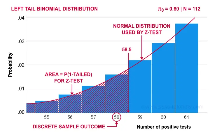
The reason for the continuity correction is that the number of successes strictly follows a binomial distribution. This discrete distribution gives the exact probability for each separate outcome.

When approximating these probabilities with a probability density function -such as the normal distribution- we need to include the entire outcome. This runs from (outcome - 0.5) to (outcome + 0.5) as illustrated below for our example.

Finally, the screenshot below shows the SPSS output for the (un)corrected z-tests.

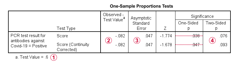
“Test Value” refers to $\pi_0$, the hypothesized population proportion;

“Observed Test Value” refers to $pi - \pi_0$;

SPSS reports the wrong standard error for this test;

the z-values and p-values confirm our calculations.

Confidence Interval for Single Proportion

Computing a confidence interval for a proportion uses a different standard error than the corresponding z-test:

$$SE_a = \sqrt{\frac{pi(1 - pi)}{N}}$$

Note that the standard error now uses our sample proportion $pi$ instead of the hypothesized population proportion $\pi_0$. Our sample of $N$ = 112 came up with a proportion of 0.52 and therefore

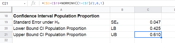
$$SE_a = \sqrt{\frac{0.52(1 - 0.52)}{112}} = 0.047.$$

We can now construct a confidence interval for the population proportion $\pi$ with

$$CI_{\pi} = pi - SE_a \cdot Z_{1-^{\alpha}_2} \lt \pi \lt pi + SE_a \cdot Z_{1-^{\alpha}_2}$$

For a 95% CI, $\alpha$ = 0.05. Therefore,

$$Z_{1-^{\alpha}_2} = Z_{.975} \approx 1.96$$

and this results in

$$CI_{\pi} = 0.52 - 0.047 \cdot 1.96 \lt \pi \lt 0.52 + 0.047 \cdot 1.96 = $$

$$CI_{\pi} = 0.43 \lt \pi \lt 0.61$$

This means that the interval [0.43,0.61] has a 95% likelihood of enclosing the population proportion of people carrying antibodies against Covid-19.

The screenshot below shows how to compute this CI in this Googlesheet.

Confidence Interval Proportion Googlesheets

Agresti-Coull Adjustment for CI

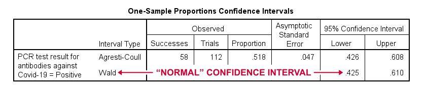
We proposed earlier that the aforementioned confidence interval requires that $n_1 \ge 15$ and $n_2 \ge 15$. Agresti & Coull (1998)¹ proposed a simple adjustment when this assumption is not met:

$n_{1ac} = n_1 + 2$ and
$n_{2ac} = n_2 + 2$.

That is, we simply add 2 observations to each group and then proceed as usual. The example presented by the authors involves a sample containing

$n_1$ = 0 respondents who own an iPod and
$n_2$ = 20 respondents who don't own an iPod.

After adding 2 observations to either group, we simply compute the confidence interval for

$n_1$ = 22 respondents don't own an iPod and
$n_2$ = 2 respondents do own an iPod.

This initially results in

$$CI_{\pi} = \frac{22}{24} - 0.056 \cdot 1.96 \lt \pi \lt \frac{22}{24} + 0.056 \cdot 1.96 = $$

$$CI_{\pi} = 0.807 \lt \pi \lt 1.027$$

However, since proportions can't be larger than 1, we'll censor this interval to [0.807,1.000].

The screenshot below shows the SPSS output for (un)adjusted confidence intervals for our Covid-19 example.

SPSS Confidence Interval Single Proportion Output

Relation to Other Tests

First off, the z-test for a single proportion without the continuity correction is equivalent to the chi-square goodness-of-fit test: these tests always yield identical p-values.

Second, the z-test for a single proportion with the continuity correction comes very close to the binomial test: for our Covid-19 example,

p(2-tailed) = .093 for the continuity corrected z-test;
2 · p(1-tailed) = .095 for the binomial test.

Note that a binomial test yields an exact p-value for some sample proportion. However, some reasons for not using it are that

it only yields 1-tailed p-values unless $\pi$ = 0.50;
it does not yield any confidence intervals;
it is computationally intensive for larger sample sizes.

References

Agresti, A. & Coull, B.A. (1998). Approximate Is Better than "Exact" for Interval Estimation of Binomial Proportions The American Statistician, 52(2), 119-126.
Agresti, A. & Franklin, C. (2014). Statistics. The Art & Science of Learning from Data. Essex: Pearson Education Limited.
Van den Brink, W.P. & Koele, P. (1998). Statistiek, deel 2 [Statistics, part 2]. Amsterdam: Boom.
Van den Brink, W.P. & Koele, P. (2002). Statistiek, deel 3 [Statistics, part 3]. Amsterdam: Boom.
Twisk, J.W.R. (2016). Inleiding in de Toegepaste Biostatistiek [Introduction to Applied Biostatistics]. Houten: Bohn Stafleu van Loghum.

Z-Test for 2 Independent Proportions – Quick Tutorial

Z-Test - Simple Example
Assumptions
Z-Test Formulas
Confidence Interval for the Difference between Proportions
Effect Size I - Cohen’s H
Z-Tests in Googlesheets

Definition & Introduction

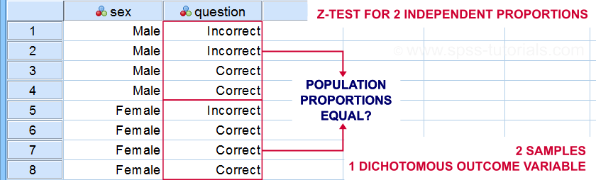
A z-test for 2 independent proportions examines
if some event occurs equally often in 2 subpopulations. Example: do equal percentages of male and female students answer some exam question correctly? The figure below sketches what the data required may look like.

Z-Test - Simple Example

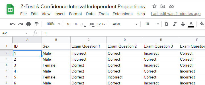
A simple random sample of n = 175 male and n = 164 female students completed 5 exam questions. The raw data -partly shown below- are in this Googlesheet (read-only).

Z Test Independent Proportions Example Data

Let's look into exam question 1 first. The raw data on this question can be summarized by the contingency table shown below.

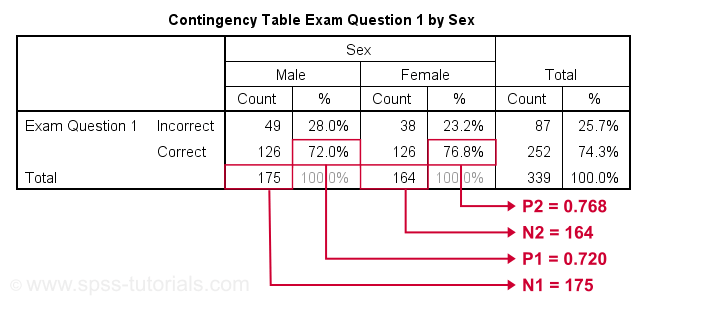
Right, so our contingency table shows the percentages of male and female respondents who answered question 1 correctly. In statistics, however, we usually prefer proportions over percentages. Summarizing our findings, we see that

a proportion of p1 = 0.720 out of n1 = 175 male students and
a proportion of p2 = 0.768 out of n2 = 164 female students answered correctly.

In our sample, female students did slightly better than male students. However, sample outcomes typically differ somewhat
from their population counterparts. Even if the entire male and female populations perform similarly, we may still find a small sample difference. This could easily result from drawing random samples of students. The z-test attempts to nullify this hypothesis and thus demonstrate that the populations really do perform differently.

Null Hypothesis

The null hypothesis for a z-test for independent proportions is that the difference between 2 population proportions is zero. If this is true, then the difference between the 2 sample proportions should be close to zero. Outcomes that are very different from zero are unlikely and thus argue against the null hypothesis. So exactly how unlikely is a given outcome? Computing this is fairly easy but it does require some assumptions.

Assumptions

The assumptions for a z-test for independent proportions are

independent observations and
sufficient sample sizes.

So what are sufficient sample sizes? Agresti and Franklin (2014)⁴ suggest that the test results are sufficiently accurate if

$p_a \cdot n_a \gt 10$,
$(1-p_a) \cdot n_a \gt 10$,
$p_b \cdot n_b \gt 10$,
$(1-p_b) \cdot n_b \gt 10$

where

$n_a$ and $n_b$ denote the sample sizes of groups a and b and
$p_a$ and $p_b$ denote the proportions of “successes” in both groups.

Z-Test Formulas

For computing our z-test, we first simply compute the difference between our sample proportions as

$$dif = p1 - p2$$

For our example data, this results in

$$dif = 0.720 - 0.768 = -.048.$$

Now, the null hypothesis claims that both subpopulations have the same proportion of successes. We estimate this as

$$\hat{p} = \frac{p_a\cdot n_a + p_b\cdot n_b}{n_a + n_b}$$

where $\hat{p}$ is the estimated proportion for both subpopulations. Note that this is simply the proportion of successes for both samples lumped together. For our example data, that'll be

$$\hat{p} = \frac{0.720\cdot 175 + 0.768\cdot 164}{175 + 164} = 0.743$$

Next up, the standard error for the difference under H₀ is

$$SE_0 = \sqrt{\hat{p}\cdot (1-\hat{p})\cdot(\frac{1}{n_a} + \frac{1}{n_b})}$$

For our example, that'll be

$$SE_0 = \sqrt{0.743\cdot (1-0.743)\cdot(\frac{1}{175} + \frac{1}{164})} = .0475$$

We can now readily compute our test statistic $Z$ as

$$Z = \frac{dif}{SE_0}$$

For our example, that'll be

$$Z = \frac{-.048}{.0475} = -1.02$$

If the z-test assumptions are met, then $Z$ approximately follows a standard normal distribution. From this we can readily look up that

$$P(Z\lt -1.02) = 0.155$$

so our 2-tailed significance is

$$P(2-tailed) = 0.309$$

Conclusion: we don't reject the null hypothesis. If the population difference is zero, then finding the observed sample difference or a more extreme one is pretty likely. Our data don't contradict the claim of male and female student populations performing equally on exam question 1.

Confidence Interval for the Difference between Proportions

Our data show that the difference between our sample proportions, $dif$ = -.048. The percentage of males who answered correctly is some 4.8% lower than that of females.

However, since our 4.8% is only based on a sample, it's likely to be somewhat “off”. So precisely how much do we expect it to be “off”? We can answer this by computing a confidence interval.

First off, we now assume an alternative hypothesis $H_A$ that the population difference is -.048. The standard error is now computed slightly differently than under $H_0$:

$$SE_A = \sqrt{\frac{p_a (1 - p_a)}{n_a} + \frac{p_b (1 - p_b)}{n_b}}$$

For our example data, that'll be

$$SE_A = \sqrt{\frac{.72 (1 - .72)}{175} + \frac{.77 (1 - .77)}{164}} = 0.0473$$

Now, the confidence interval for the population difference $\delta$ between the proportions is

$$CI_{\delta} = \hat{p} - SE_A \cdot Z_{1-^{\alpha}_2} \lt \delta \lt \hat{p} + SE_A \cdot Z_{1-^{\alpha}_2}$$

For a 95% CI, $\alpha$ = 0.05. Therefore,

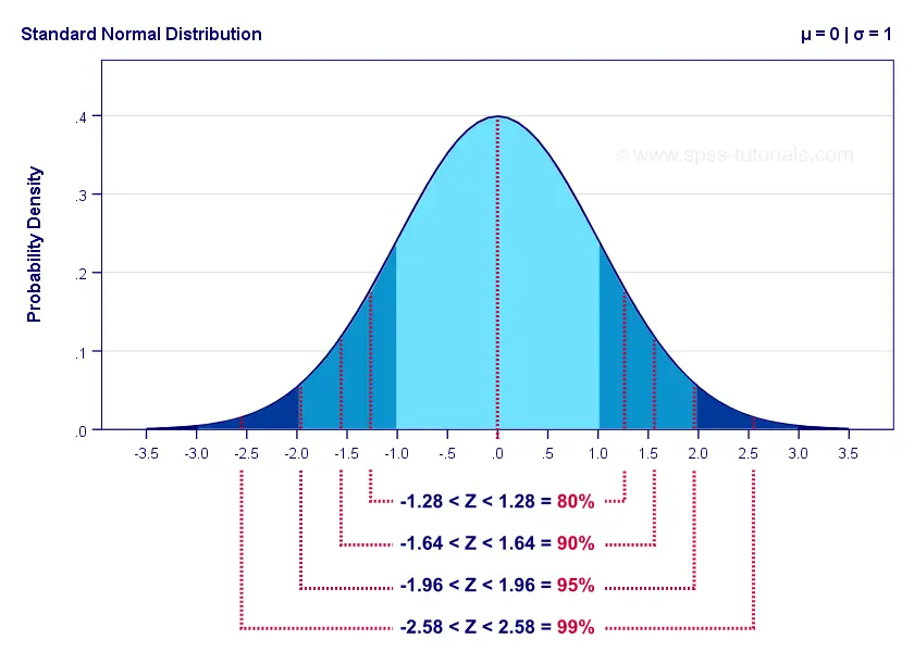
$$Z_{1-^{\alpha}_2} = Z_{.975} \approx 1.96$$

The figure below illustrates these and some other critical z-values for different $\alpha$ levels. The exact values can easily be looked up in Excel or Googlesheets as shown in Normal Distribution - Quick Tutorial.

Standard Normal Distribution With Critical Values

For our example, the 95% confidence interval is

$$CI_{\delta} = -.048 - .0473 \cdot 1.96 \lt \delta \lt -.048 + .0473 \cdot 1.96 =$$

$$CI_{\delta} = -.141 \lt \delta \lt 0.044$$

That is, there's a 95% likelihood that the population difference lies between -.141 and .044. Note that this CI contains zero: a zero difference between the population proportions -meaning that males and females perform equally well- is within a likely range.

Effect Size I - Cohen’s H

Our sample proportions are p1 = 0.72 and p2 = 0.77. Should we consider that a small, medium or large effect? A likely effect size measure is simply the difference between our proportions. However, a more suitable measure is Cohen’s H, defined as $$h = |\;2\cdot arcsin\sqrt{p1} - 2\cdot arcsin\sqrt{p2}\;|$$
where $arcsin$ refers to the arcsine function.

Basic rules of thumb⁷ are that

h = 0.2 indicates a small effect;
h = 0.5 indicates a medium effect;
h = 0.8 indicates a large effect.

For our example data, Cohen’s H is
$$h = |\;2\cdot arcsin\sqrt{0.72} - 2\cdot arcsin\sqrt{0.77}\;|$$
$$h = |\;2\cdot 1.01 - 2\cdot 1.07\;| = 0.11$$
Our rules of thumb suggest that this effect is close to negligible.

Effect Size II - Phi Coefficient

An alternative effect size measure for the z-test for independent proportions is the phi coefficient, denoted by φ (the Greek letter “phi”). This is simply a Pearson correlation between dichotomous variables.

Following the rules of thumb for correlations⁷, we could propose that

$|\;\phi\;| = 0.1$ indicates a small effect;
$|\;\phi\;| = 0.3$ indicates a medium effect;
$|\;\phi\;| = 0.5$ indicates a large effect.

However, we feel these rules of thumb are clearly disputable: they may be overly strict because | φ | tends to be considerably smaller than | r |.

Z-Tests in Googlesheets

Z-tests were only introduced to SPSS version 27 in 2020. They're completely absent from some other statistical packages such as JASP. We therefore developed this Googlesheet (read-only), partly shown below.

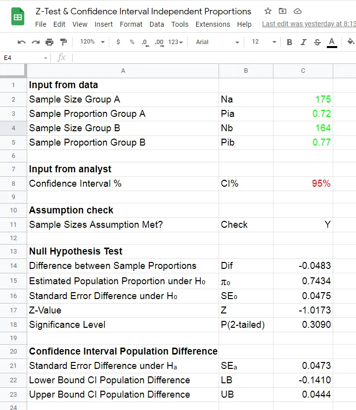
Z-Test Independent Proportions Googlesheets Calculator

You can download this sheet as Excel and use it as a fast and easy z-test calculator. Given 2 sample proportions and 2 sample sizes, our tool

checks if the sample size assumption is met;
computes the 2-tailed-significance-level for the z-test;
computes a confidence interval for the difference between the proportions;

We prefer this tool over online calculators because

results in Excel can (and should) be saved with any other project files whereas results from online calculators usually aren't;
all formulas used in Excel are visible and can thus be verified;
running many z-tests in Excel can be done effortlessly be expanding the formula section.

SPSS users can readily create the exact right input for the Excel tool with a MEANS command as illustrated by the SPSS syntax below:

*Create table with sample sizes and proportions for v1 to v5 by sex.

means v1 to v5 by sex
/cells count mean.

Doing so for 2+ dependent variables results in a table as shown below.

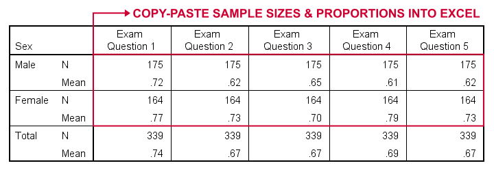
SPSS Means Ouput Table For Z Test Excel Tool

Note that all dependent variables must follow a 0-1 coding in order for this to work.

Relation Z-Test with Other Tests

An alternative for the z-test for independent proportions is a chi-square independence test. The significance level of the latter (which is always 1-tailed) is identical to the 2-tailed significance of the former.

Upon closer inspection, these tests -as well as their assumptions- are statistically equivalent. However, there's 2 reasons for preferring the z-test over the chi-square test:

the z-test yields a confidence interval for the difference between the proportions;
running 2 or more z-tests is easier and results in a clearer output table than 2(+) contingency tables with chi-square tests.

Second, the z-test for independent proportions is asymptotically equivalent to the independent samples t-test: their results become more similar insofar as larger sample sizes are used. But -reversely- t-test results for proportions are “off” more insofar as sample sizes are smaller.
Other reasons for preferring the z-test over the t-test are that

the z-test results in higher power and smaller confidence intervals insofar as smaller sample sizes are used;
the t-test requires normally distributed dependent variables and equal population-variances whereas the z-test doesn't.

So -in short- use a z-test when appropriate. Your statistical package not including it is a poor excuse for not doing what's right.

Thanks for reading.

References

Van den Brink, W.P. & Koele, P. (1998). Statistiek, deel 2 [Statistics, part 2]. Amsterdam: Boom.
Van den Brink, W.P. & Koele, P. (2002). Statistiek, deel 3 [Statistics, part 3]. Amsterdam: Boom.
Warner, R.M. (2013). Applied Statistics (2nd. Edition). Thousand Oaks, CA: SAGE.
Agresti, A. & Franklin, C. (2014). Statistics. The Art & Science of Learning from Data. Essex: Pearson Education Limited.
Howell, D.C. (2002). Statistical Methods for Psychology (5th ed.). Pacific Grove CA: Duxbury.
Slotboom, A. (1987). Statistiek in woorden [Statistics in words]. Groningen: Wolters-Noordhoff.
Cohen, J (1988). Statistical Power Analysis for the Social Sciences (2nd. Edition). Hillsdale, New Jersey, Lawrence Erlbaum Associates.

Z-Scores – What and Why?

Quick Definition

Z-scores are scores that have mean = 0
and standard deviation = 1. Z-scores are also known as standardized scores because they are scores that have been given a common standard. This standard is a mean of zero and a standard deviation of 1.

Contrary to what many people believe, z-scores are not necessarily normally distributed.

Z-Scores - Example

A group of 100 people took some IQ test. My score was 5. So is that good or bad? At this point, there's no way of telling because we don't know what people typically score on this test. However, if my score of 5 corresponds to a z-score of 0.91, you'll know it was pretty good: it's roughly a standard deviation higher than the average (which is always zero for z-scores).
What we see here is that standardizing scores facilitates the interpretation of a single test score. Let's see how that works.

Scores - Histogram

A quick peek at some of our 100 scores on our first IQ test shows a minimum of 1 and a maximum of 6. However, we'll gain much more insight into these scores by inspecting their histogram as shown below.

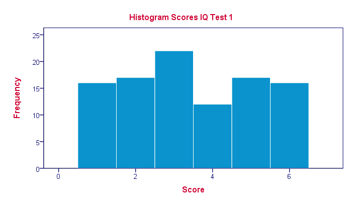
The histogram confirms that scores range from 1 through 6 and each of these scores occurs about equally frequently. This pattern is known as a uniform distribution and we typically see this when we roll a die a lot of times: numbers 1 through 6 are equally likely to come up. Note that these scores are clearly not normally distributed.

Z-Scores - Standardization

We suggested earlier on that giving scores a common standard of zero mean and unity standard deviation facilitates their interpretation. We can do just that by

first subtracting the mean over all scores from each individual score and
then dividing each remainder by the standard deviation over all scores.

These two steps are the same as the following formula:
$$Z_x = \frac{X_i - \overline{X}}{S_x}$$
As shown by the table below, our 100 scores have a mean of 3.45 and a standard deviation of 1.70. 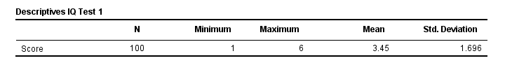Z-Scores Descriptive Statistics By entering these numbers into the formula, we see why a score of 5 corresponds to a z-score of 0.91:
$$Z_x = \frac{5 - 3.45}{1.70} = 0.91$$
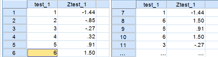
In a similar vein, the screenshot below shows the z-scores for all distinct values of our first IQ test added to the data. Z-Scores Added to Data

Z-Scores - Histogram

In practice, we obviously have some software compute z-scores for us. We did so and ran a histogram on our z-scores, which is shown below. Z-Scores Uniform Distribution If you look closely, you'll notice that the z-scores indeed have a mean of zero and a standard deviation of 1. Other than that, however, z-scores follow the exact same distribution as original scores. That is, standardizing scores doesn't make their distribution more “normal” in any way.

What's a Linear Transformation?

Z-scores are linearly transformed scores. What we mean by this, is that if we run a scatterplot of scores versus z-scores, all dots will be exactly on a straight line (hence, “linear”). The scatterplot below illustrates this. It contains 100 points but many end up right on top of each other.

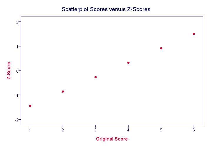
Z-Scores Scatterplot Scores Versus Z-Scores

In a similar vein, if we had plotted scores versus squared scores, our line would have been curved; in contrast to standardizing, taking squares is a non linear transformation.

Z-Scores and the Normal Distribution

We saw earlier that standardizing scores doesn't change the shape of their distribution in any way; distribution don't become any more or less “normal”. So why do people relate z-scores to normal distributions?

The reason may be that many variables actually do follow normal distributions. Due to the central limit theorem, this holds especially for test statistics. If a normally distributed variable is standardized, it will follow a standard normal distribution.

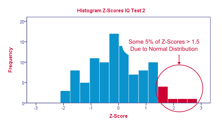
This is a common procedure in statistics because values that (roughly) follow a standard normal distribution are easily interpretable. For instance, it's well known that some 2.5% of values are larger than two and some 68% of values are between -1 and 1.

The histogram below illustrates this: if a variable is roughly normally distributed, z-scores will roughly follow a standard normal distribution. For z-scores, it always holds (by definition) that a score of 1.5 means “1.5 standard deviations higher than average”. However, if a variable also follows a standard normal distribution, then we also know that 1.5 roughly corresponds to the 95th percentile.

Z-Scores in SPSS

SPSS users can easily add z-scores to their data by using a DESCRIPTIVES command as in descriptives test_1 test_2/save. in which “save” means “save z-scores as new variables in my data”. For more details, see z-scores in SPSS.