SPSS Chi-Square Test with Pairwise Z-Tests

Most data analysts are familiar with post hoc tests for ANOVA. Oddly, post hoc tests for the chi-square independence test are not widely used. This tutorial walks you through 2 options for obtaining and interpreting them in SPSS.

• Option 1 - CROSSTABS
• CROSSTABS with Pairwise Z-Tests Output
• Option 2 - Custom Tables
• Custom Tables with Pairwise Z-Tests Output
• Can these Z-Tests be Replicated?

Example Data

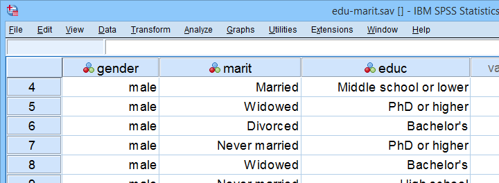
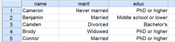
A sample of N = 300 respondents were asked about their education level and marital status. The data thus obtained are in edu-marit.sav. All examples in this tutorial use this data file.

Chi-Square Independence Test

Right. So let's see if education level and marital status are associated in the first place: we'll run a chi-square independence test with the syntax below. This also creates a contingency table showing both frequencies and column percentages.

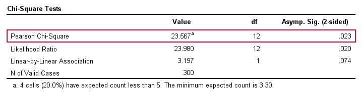
Let's first take a look at the actual test results shown below.

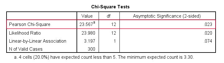
First off, we reject the null hypothesis of independence: education level and marital status are associated, χ²(12) = 23.57, p = 0.023. Note that that SPSS wrongfully reports this 1-tailed significance as a 2-tailed significance. But anyway, what we really want to know is precisely which percentages differ significantly from each other?

Option 1 - CROSSTABS

We'll answer this question by slightly modifying our syntax: adding BPROP (short for “Bonferroni proportions”) to the /CELLS subcommand does the trick.

Running this simple syntax results in the table shown below.

CROSSTABS with Pairwise Z-Tests Output

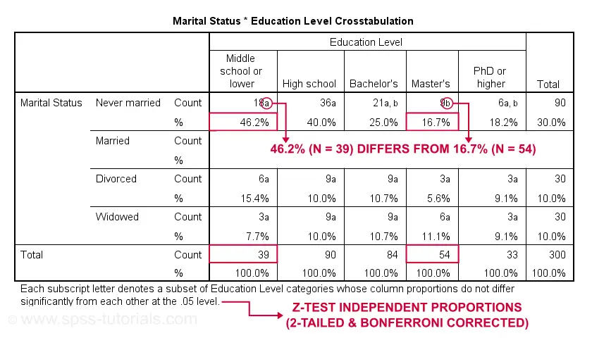
First off, take a close look at the table footnote: “Each subscript letter denotes a subset of Education Level categories whose column proportions do not differ significantly from each other at the .05 level.”
These conclusions are based on z-tests for independent proportions. These also apply to the percentages shown in the table: within each row, each possible pair of percentages is compared using a z-test. If they don't differ, they get a similar subscript. Reversely, within each row, percentages that don't share a subscript
are significantly different. For example, the percentage of people with middle school who never married is 46.2% and its frequency of n = 18 is labeled “a”. For those with a Master’s degree, 16.7% never married and its frequency of 9 is not labeled “a”. This means that 46.2% differs significantly from 16.7%.

The frequency of people with a Bachelor’s degree who never married (n = 21 or 25.0%) is labeled both “a” and “b”. It doesn't differ significantly from any cells labeled “a”, “b” or both. Which are all cells in this table row.

Now, a Bonferroni correction is applied for the number of tests within each row. This means that for \(k\) columns,
$$P_{bonf} = P\cdot\frac{k(k - 1)}{2}$$
where

• \(P_{bonf}\) denotes a Bonferroni corrected p-value and
• \(P\) denotes a “normal” (uncorrected) p-value.

Right, now our table has 5 education levels as columns so $$P_{bonf} = P\cdot\frac{5(5 - 1)}{2} = P \cdot 10$$
which means that each p-value is multiplied by 10 and only then compared to alpha = 0.05. Or -reversely- only z-tests yielding an uncorrected p < 0.005 are labeled “significant”. This holds for all tests reported in this table. I'll verify these claims later on.

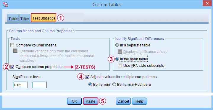
Option 2 - Custom Tables

A second option for obtaining “post hoc tests” for chi-square tests are Custom Tables. They're found under Analyze Tables Custom Tables but only if you have a Custom Tables license. The figure below suggests some basic steps.

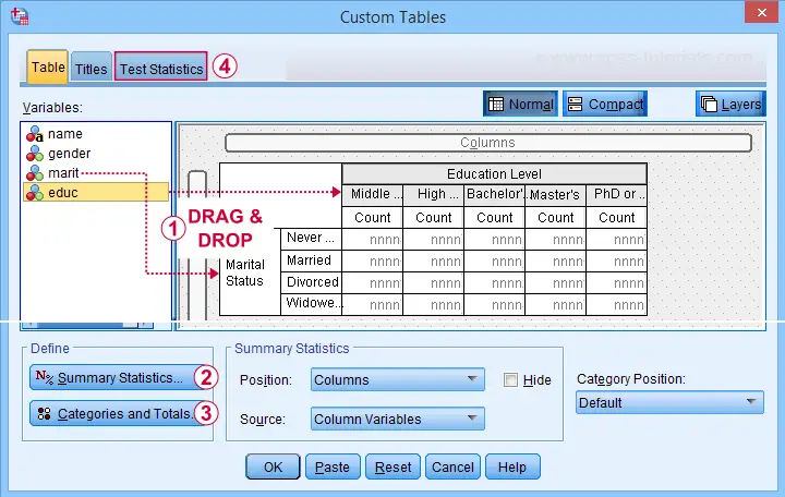
You probably want to select both frequencies and column percentages for education level.
We recommend you add totals for education levels as well.

Next, our z-tests are found in the Test Statistics tab shown below.

Completing these steps results in the syntax below.

Custom Tables with Pairwise Z-Tests Output

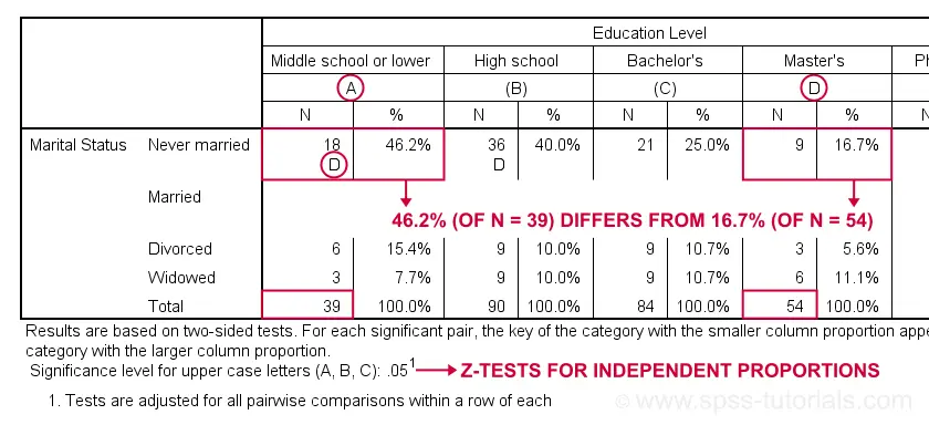
Let's first try and understand what the footnote says: “Results are based on two-sided tests. For each significant pair, the key of the category with the smaller column proportion appears in the category with the larger column proportion. Significance level for upper case letters (A, B, C): .05. Tests are adjusted for all pairwise comparisons within a row of each innermost subtable using the Bonferroni correction.”

Now, for normal 2-way contingency tables, the “innermost subtable” is simply the entire table. Within each row, each possible pair of column proportions is compared using a z-test. If 2 proportions differ significantly, then the higher is flagged with the column letter of the lower. Somewhat confusingly, SPSS flags the frequencies instead of the percentages.

In the first row (never married), the D in column A indicates that these 2 percentages
differ significantly: the percentage of people who never married is significantly higher for those who only completed middle school (46.2% from n = 39) than for those who completed a Master’s degree (16.7% from n = 54).

Again, all z-tests use α = 0.05 after Bonferroni correcting their p-values for the number of columns in the table. For our example table with 5 columns, each p-value is multiplied by \(0.5\cdot5(5 - 1) = 10\) before evaluating if it's smaller than the chosen alpha level of 0.05.

Can these Z-Tests be Replicated?

Yes. They can.

Custom Tables has an option to create a table containing the exact p-values for all pairwise z-tests. It's found in the Test Statistics tab. Selecting it results in the syntax below.

Exact P-Values for Z-Tests

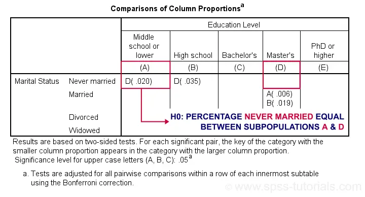
For the first row (never married), SPSS claims that the Bonferroni corrected p-value for comparing column percentages A and D is p = 0.020. For our example table, this implies an uncorrected p-value of p = 0.0020.
We replicated this result with an Excel z-test calculator. Taking the Bonferroni correction into account, it comes up with the exact same p-value as SPSS.

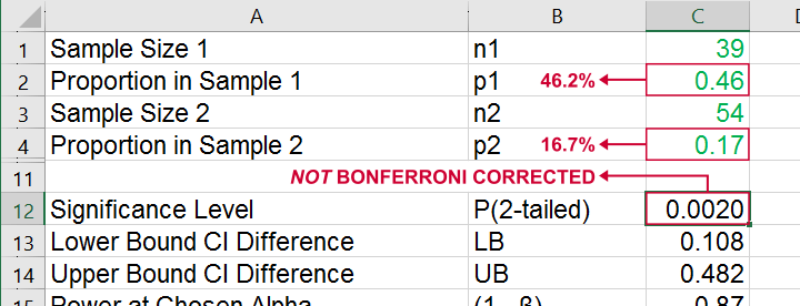
All other p-values reported by SPSS were also exactly replicated by our Excel calculator.

I hope this tutorial has been helpful for obtaining and understanding pairwise z-tests for contingency tables. If you've any questions or feedback, please throw us a comment below.

Thanks for reading!

Chi-Square Goodness-of-Fit Test – Simple Tutorial

• Null Hypothesis
• Assumptions
• Formulas
• Effect Size - Cohen’s W
• Power and Sample Size Calculation

A chi-square goodness-of-fit test examines if a categorical variable
has some hypothesized frequency distribution in some population. The chi-square goodness-of-fit test is also known as

• one-sample chi-square test (SPSS) or
• multinomial test (JASP).

Example - Testing Car Advertisements

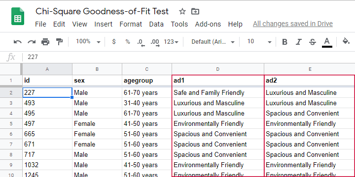
A car manufacturer wants to launch a campaign for a new car. They'll show advertisements -or “ads”- in 4 different sizes. For ad each size, they have 4 ads that try to convey some message such as “this car is environmentally friendly”. They then asked N = 80 people which ad they liked most. The data thus obtained are in this Googlesheet, partly shown below.

So which ads performed best in our sample? Well, we can simply look up which ad was preferred by most respondents: the ad having the highest frequency is the mode for each ad size.

So let's have a look at the frequency distribution for the first ad size -ad1- as visualized in the bar chart shown below.

Observed Frequencies and Bar Chart

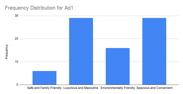
The observed frequencies shown in this chart are

1. Safe and Family Friendly: 6
2. Luxurious and Masculine: 29
3. Environmentally Friendly: 16
4. Spacious and Convenient: 29

Note that ad1 has a bimodal distribution: ads 2 and 4 are both winners with 29 votes. However, our data only hold a sample of N = 80. So can we conclude that ads 2 and 4
also perform best in the entire population? The chi-square goodness-of-fit answers just that. And for this example, it does so by trying to reject the null hypothesis that all ads perform equally well in the population.

Null Hypothesis

Generally, the null hypothesis for a chi-square goodness-of-fit test is simply

$$H_0: P_{01}, P_{02},...,P_{0m},\; \sum_{i=0}^m\biggl(P_{0i}\biggr) = 1$$

where \(P_{0i}\) denote population proportions for \(m\) categories in some categorical variable. You can choose any set of proportions as long as they add up to one. In many cases, all proportions being equal is the most likely null hypothesis.
For a dichotomous variable having only 2 categories, you're better off using

• a binomial test because it gives the exact instead of the approximate significance level or
• a z-test for 1 proportion because it gives a confidence interval for the population proportion.

Anyway, for our example, we'd like to show that some ads perform better than others. So we'll try to refute that our 4 population proportions are all equal and -hence- 0.25.

Expected Frequencies

Now, if the 4 population proportions really are 0.25 and we sample N = 80 respondents, then we expect each ad to be preferred by 0.25 · 80 = 20 respondents. That is, all 4 expected frequencies are 20. We need to know these expected frequencies for 2 reasons:

• computing our test statistic requires expected frequencies and
• the assumptions for the chi-square goodness-of-fit test involve expected frequencies as well.

Assumptions

The chi-square goodness-of-fit test requires 2 assumptions^2,3:

1. independent observations;
2. for 2 categories, each expected frequency \(Ei\) must be at least 5.
   For 3+ categories, each \(Ei\) must be at least 1 and no more than 20% of all \(Ei\) may be smaller than 5.

The observations in our data are independent because they are distinct persons who didn't interact while completing our survey. We also saw that all \(Ei\) are (0.25 · 80 =) 20 for our example. So this second assumption is met as well.

Formulas

We'll first compute the \(\chi^2\) test statistic as

$$\chi^2 = \sum\frac{(O_i - E_i)^2}{E_i}$$

where

• \(O_i\) denotes the observed frequencies and
• \(E_i\) denotes the expected frequencies -usually all equal.

For ad1, this results in

$$\chi^2 = \frac{(16 - 20)^2}{20} + \frac{(29 - 20)^2}{20} + \frac{(9 - 20)^2}{20} + \frac{(29 - 20)^2}{20} = 18.7 $$

If all assumptions have been met, \(\chi^2\) approximately follows a chi-square distribution with \(df\) degrees of freedom where

$$df = m - 1$$

for \(m\) frequencies. Since we have 4 frequencies for 4 different ads,

$$df = 4 - 1 = 3$$

for our example data. Finally, we can simply look up the significance level as

$$P(\chi^2(3) > 18.7) \approx 0.00032$$

We ran these calculations in this Googlesheet shown below.

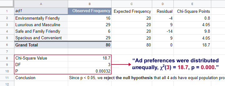
So what does this mean? Well, if all 4 ads are equally preferred in the population, there's a 0.00032 chance of finding our observed frequencies. Since p < 0.05, we reject the null hypothesis. Conclusion: some ads are preferred by more people than others in the entire population of readers.

Right, so it's safe to assume that the population proportions are not all equal. But precisely how different are they? We can express this in a single number: the effect size.

Effect Size - Cohen’s W

The effect size for a chi-square goodness-of-fit test -as well as the chi-square independence test- is Cohen’s W. Some rules of thumb¹ are that

• Cohen’s W = 0.10 indicates a small effect size;
• Cohen’s W = 0.30 indicates a medium effect size;
• Cohen’s W = 0.50 indicates a large effect size.

Cohen’s W is computed as

$$W = \sqrt{\sum_{i = 1}^m\frac{(P_{oi} - P_{ei})^2}{P_{ei}}}$$

where

• \(P_{oi}\) denote observed proportions and
• \(P_{ei}\) denote expected proportions under the null hypothesis for
• \(m\) cells.

For ad1, the null hypothesis states that all expected proportions are 0.25. The observed proportions are computed from the observed frequencies (see screenshot below) and result in

$$W = \sqrt{\frac{(0.2 - 0.25)^2}{0.25} +\frac{(0.3625 - 0.25)^2}{0.25} +\frac{(0.075 - 0.25)^2}{0.25} +\frac{(0.3625 - 0.25)^2}{0.25} } = $$

$$W = \sqrt{0.234} = 0.483$$

We ran these computations in this Googlesheet shown below.

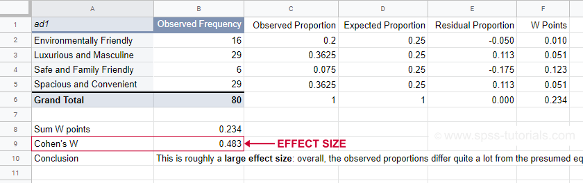
For ad1, the effect size \(W\) = 0.483. This indicates a large overall difference between the observed and expected frequencies.

Power and Sample Size Calculation

Now that we computed our effect size, we're ready for our last 2 steps. First off, what about power? What's the probability demonstrating an effect if

• we test at α = 0.05;
• we have a sample of N = 80;
• df = 3 (our outcome variable has 4 categories);
• we don't know the population effect size \(W\)?

The chart below -created in G*Power- answers just that.

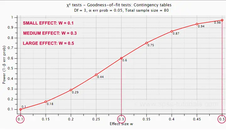
Some basic conclusions are that

• power = 0.98 for a large effect size;
• power = 0.60 for a medium effect size;
• power = 0.10 for a small effect size.

These outcomes are not too great: we only have a 0.60 probability of rejecting the null hypothesis if the population effect size is medium and N = 80. However, we can increase power by increasing the sample size. So which sample sizes do we need if

• we test at α = 0.05;
• we want to have power = 0.80;
• df = 3 (our outcome variable has 4 categories);
• we don't know the population effect size \(W\)?

The chart below shows how required sample sizes decrease with increasing effect sizes.

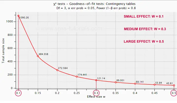
Under the aforementioned conditions, we have power ≥ 0.80

• for a large effect size if N = 44;
• for a medium effect size if N = 122;
• for a small effect size if N = 1091.

References

1. Cohen, J (1988). Statistical Power Analysis for the Social Sciences (2nd. Edition). Hillsdale, New Jersey, Lawrence Erlbaum Associates.
2. Siegel, S. & Castellan, N.J. (1989). Nonparametric Statistics for the Behavioral Sciences (2nd ed.). Singapore: McGraw-Hill.
3. Warner, R.M. (2013). Applied Statistics (2nd. Edition). Thousand Oaks, CA: SAGE.

Chi-Square Independence Test – What and Why?

• Chi-Square Independence Test - What Is It?
• Null Hypothesis
• Assumptions
• Test Statistic
• Effect Size
• Reporting

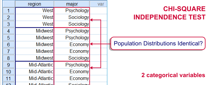
Chi-Square Independence Test - What Is It?

The chi-square independence test evaluates if
two categorical variables are related in some population. Example: a scientist wants to know if education level and marital status are related for all people in some country. He collects data on a simple random sample of n = 300 people, part of which are shown below.

Chi-Square Test - Observed Frequencies

A good first step for these data is inspecting the contingency table of marital status by education. Such a table -shown below- displays the frequency distribution of marital status for each education category separately. So let's take a look at it.

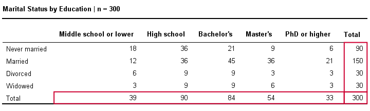
The numbers in this table are known as the observed frequencies. They tell us an awful lot about our data. For instance,

• there's 4 marital status categories and 5 education levels;
• we succeeded in collecting data on our entire sample of n = 300 respondents (bottom right cell);
• we've 84 respondents with a Bachelor’s degree (bottom row, middle);
• we've 30 divorced respondents (last column, middle);
• we've 9 divorced respondents with a Bachelor’s degree.

Chi-Square Test - Column Percentages

Although our contingency table is a great starting point, it doesn't really show us if education level and marital status are related. This question is answered more easily from a slightly different table as shown below.

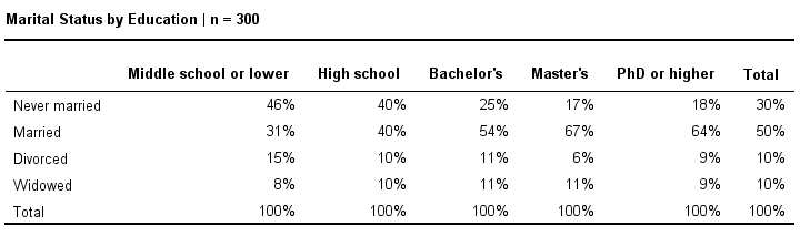
This table shows -for each education level separately- the percentages of respondents that fall into each marital status category. Before reading on, take a careful look at this table and tell me is marital status related to education level and -if so- how? If we inspect the first row, we see that 46% of respondents with middle school never married. If we move rightwards (towards higher education levels), we see this percentage decrease: only 18% of respondents with a PhD degree never married (top right cell).

Reversely, note that 64% of PhD respondents are married (second row). If we move towards the lower education levels (leftwards), we see this percentage decrease to 31% for respondents having just middle school. In short, more highly educated respondents marry more often than less educated respondents.

Chi-Square Test - Stacked Bar Chart

Our last table shows a relation between marital status and education. This becomes much clearer by visualizing this table as a stacked bar chart, shown below.

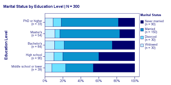
If we move from top to bottom (highest to lowest education) in this chart, we see the dark blue bar (never married) increase. Marital status is clearly associated with education level.The lower someone’s education, the smaller the chance he’s married. That is: education “says something” about marital status (and reversely) in our sample. So what about the population?

Chi-Square Test - Null Hypothesis

The null hypothesis for a chi-square independence test is that two categorical variables are independent in some population. Now, marital status and education are related -thus not independent- in our sample. However, we can't conclude that this holds for our entire population. The basic problem is that samples usually differ from populations.

If marital status and education are perfectly independent in our population, we may still see some relation in our sample by mere chance. However, a strong relation in a large sample is extremely unlikely and hence refutes our null hypothesis. In this case we'll conclude that the variables were not independent in our population after all.

So exactly how strong is this dependence -or association- in our sample? And what's the probability -or p-value- of finding it if the variables are (perfectly) independent in the entire population?

Chi-Square Test - Statistical Independence

Before we continue, let's first make sure we understand what “independence” really means in the first place. In short, independence means that one variable doesn't
“say anything” about another variable. A different way of saying the exact same thing is that independence means that the relative frequencies of one variable
are identical over all levels of some other variable. Uh... say again? Well, what if we had found the chart below?

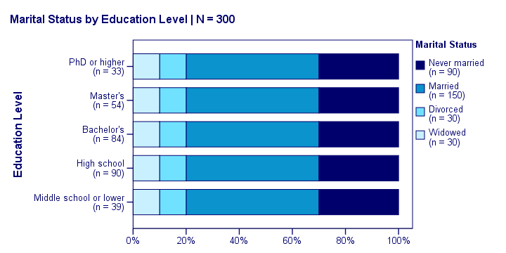
What does education “say about” marital status? Absolutely nothing! Why? Because the frequency distributions of marital status are identical over education levels: no matter the education level, the probability of being married is 50% and the probability of never being married is 30%.

In this chart, education and marital status are perfectly independent. The hypothesis of independence tells us which frequencies we should have found in our sample: the expected frequencies.

Expected Frequencies

Expected frequencies are the frequencies we expect in a sample
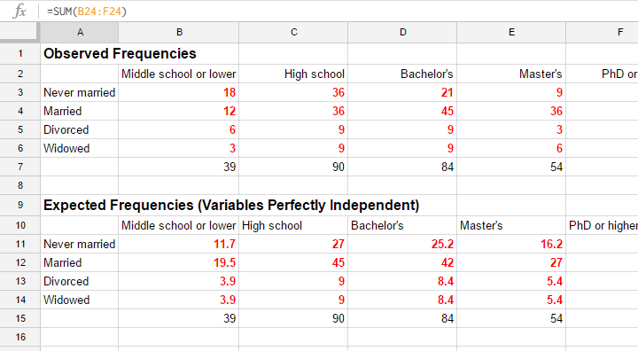
if the null hypothesis holds. If education and marital status are independent in our population, then we expect this in our sample too. This implies the contingency table -holding expected frequencies- shown below.

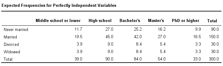
These expected frequencies are calculated as $$eij = \frac{oi\cdot oj}{N}$$
where

• \(eij\) is an expected frequency;
• \(oi\) is a marginal column frequency;
• \(oj\) is a marginal row frequency;
• \(N\) is the total sample size.

So for our first cell, that'll be $$eij = \frac{39 \cdot 90}{300} = 11.7$$
and so on. But let's not bother too much as our software will take care of all this.

Note that many expected frequencies are non integers. For instance, 11.7 respondents with middle school who never married. Although there's no such thing as “11.7 respondents” in the real world, such non integer frequencies are just fine mathematically. So at this point, we've 2 contingency tables:

• a contingency table with observed frequencies we found in our sample;
• a contingency table with expected frequencies we should have found in our sample if the variables are really independent.

The screenshot below shows both tables in this GoogleSheet (read-only). This sheet demonstrates all formulas that are used for this test.

Residuals

Insofar as the observed and expected frequencies differ, our data deviate more from independence. So how much do they differ? First off, we subtract each expected frequency from each observed frequency, resulting in a residual. That is, $$rij = oij - eij$$
For our example, this results in (5 * 4 =) 20 residuals. Larger (absolute) residuals indicate a larger difference between our data and the null hypothesis. We basically add up all residuals, resulting in a single number: the χ² (pronounce “chi-square”) test statistic.

Test Statistic

The chi-square test statistic is calculated as
$$\chi^2 = \Sigma{\frac{(oij - eij)^2}{eij}}$$
so for our data $$\chi^2 = \frac{(18 - 11.7)^2}{11.7} + \frac{(36 - 27)^2}{27} + ... + \frac{(6 - 5.4)^2}{5.4} = 23.57$$

Again, our software will take care of all this. But if you'd like to see the calculations, take a look at this GoogleSheet.

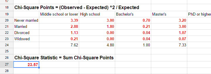
So χ² = 23.57 in our sample. This number summarizes the difference between our data and our independence hypothesis. Is 23.57 a large value? What's the probability of finding this? Well, we can calculate it from its sampling distribution but this requires a couple of assumptions.

Chi-Square Test Assumptions

The assumptions for a chi-square independence test are

1. independent observations. This usually -not always- holds if each case in SPSS holds a unique person or other statistical unit. Since this is the case for our data, we'll assume this has been met.
2. For a 2 by 2 table, all expected frequencies > 5.However, for a 2 by 2 table, a z-test for 2 independent proportions is preferred over the chi-square test.
   
   For a larger table, all expected frequencies > 1 and no more than 20% of all cells may have expected frequencies < 5.

If these assumptions hold, our χ² test statistic follows a χ² distribution. It's this distribution that tells us the probability of finding χ² > 23.57.

Chi-Square Test - Degrees of Freedom

We'll get the p-value we're after from the chi-square distribution if we give it 2 numbers:

• the χ² value (23.57) and
• the degrees of freedom (df).

The degrees of freedom is basically a number that determines the exact shape of our distribution. The figure below illustrates this point.

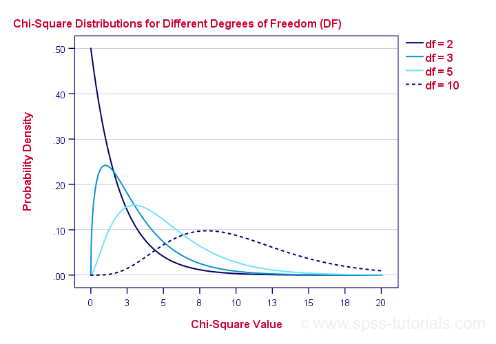
Right. Now, degrees of freedom -or df- are calculated as $$df = (i - 1) \cdot (j - 1)$$
where

• \(i\) is the number of rows in our contingency table and
• \(j\) is the number of columns

so in our example $$df = (5 - 1) \cdot (4 - 1) = 12.$$
And with df = 12, the probability of finding χ² ≥ 23.57 ≈ 0.023.We simply look this up in SPSS or other appropriate software. This is our 1-tailed significance. It basically means, there's a 0.023 (or 2.3%) chance of finding this association in our sample if it is zero in our population.

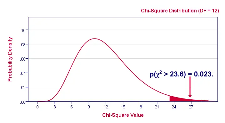
Since this is a small chance, we no longer believe our null hypothesis of our variables being independent in our population. Conclusion: marital status and education are related
in our population. Now, keep in mind that our p-value of 0.023 only tells us that the association between our variables is probably not zero. It doesn't say anything about the strength of this association: the effect size.

Effect Size

For the effect size of a chi-square independence test, consult the appropriate association measure. If at least one nominal variable is involved, that'll usually be Cramér’s V (a sort of Pearson correlation for categorical variables). In our example Cramér’s V = 0.162. Since Cramér’s V takes on values between 0 and 1, 0.162 indicates a very weak association. If both variables had been ordinal, Kendall’s tau or a Spearman correlation would have been suitable as well.

Reporting

For reporting our results in APA style, we may write something like “An association between education and marital status was observed, χ²(12) = 23.57, p = 0.023.”

Chi-Square Independence Test - Software

You can run a chi-square independence test in Excel or Google Sheets but you probably want to use a more user friendly package such as

• SPSS,
• Stata or
• SAS.

The figure below shows the output for our example generated by SPSS.

For a full tutorial (using a different example), see SPSS Chi-Square Independence Test.

Thanks for reading!

SPSS Chi-Square Independence Test Tutorial

A newly updated, ad-free video version of this tutorial
is included in our SPSS beginners course.

• Null Hypothesis
• Assumptions
• Chi-Square Independence Test in SPSS
• Output
• Reporting

Null Hypothesis for the Chi-Square Independence Test

A chi-square independence test evaluates if two categorical variables are associated in some population. We'll therefore try to refute the null hypothesis that two categorical variables are (perfectly) independent in some population. If this is true and we draw a sample from this population, then we may see some association between these variables in our sample. This is because samples tend to differ somewhat from the populations from which they're drawn.
However, a strong association between variables is unlikely to occur in a sample if the variables are independent in the entire population. If we do observe this anyway, we'll conclude that the variables probably aren't independent in our population after all. That is, we'll reject the null hypothesis of independence.

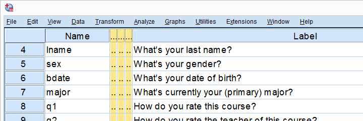
Example

A sample of 183 students evaluated some course. Apart from their evaluations, we also have their genders and study majors. The data are in course_evaluation.sav, part of which is shown below.

We'd now like to know: is study major associated with gender? And -if so- how? Since study major and gender are nominal variables, we'll run a chi-square test to find out.

Assumptions Chi-Square Independence Test

Conclusions from a chi-square independence test can be trusted if two assumptions are met:

• independent observations. This usually -not always- holds if each case in SPSS holds a unique person or other statistical unit. Since this is that case for our data, we'll assume this has been met.
• For a 2 by 2 table, all expected frequencies > 5.If you've no idea what that means, you may consult Chi-Square Independence Test - Quick Introduction. For a larger table, no more than 20% of all cells may have an expected frequency < 5 and all expected frequencies > 1.
  
  SPSS will test this assumption for us when we'll run our test. We'll get to it later.

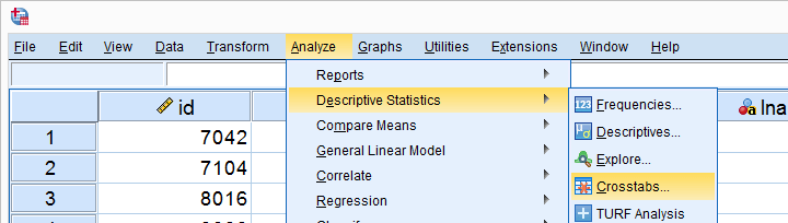
Chi-Square Independence Test in SPSS

In SPSS, the chi-square independence test is part of the CROSSTABS procedure which we can run as shown below.

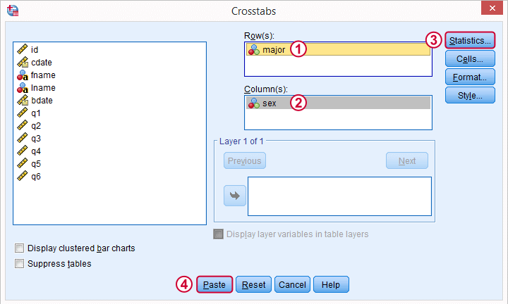
In the main dialog, we'll enter one variable into the Row(s) box and the other into Column(s). Since sex has only 2 categories (male or female), using it as our column variable results in a table that's rather narrow and high. It will fit more easily into our final report than a wider table resulting from using major as our column variable. Anyway, both options yield identical test results.
Under Stastistics we'll just select Chi-Square. Clicking Paste results in the syntax below.

SPSS Chi-Square Independence Test Syntax

You can use this syntax if you like but I personally prefer a shorter version shown below. I simply type it into the Syntax Editor window, which for me is much faster than clicking through the menu. Both versions yield identical results.

Output Chi-Square Independence Test

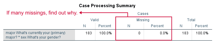
First off, we take a quick look at the Case Processing Summary to see if any cases have been excluded due to missing values. That's not the case here. With other data, if many cases are excluded, we'd like to know why and if it makes sense.

Contingency Table

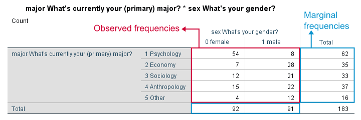
Next, we inspect our contingency table. Note that its marginal frequencies -the frequencies reported in the margins of our table- show the frequency distributions of either variable separately.
Both distributions look plausible and since there's no “no answer” categories, there's no need to specify any user missing values.

Significance Test

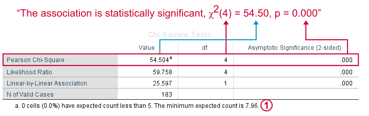
First off, our data meet the assumption of all expected frequencies > 5 that we mentioned earlier. Since this holds, we can rely on our significance test for which we use Pearson Chi-Square.
Right, we usually say that the association between two variables is statistically significant if Asymptotic Significance (2-sided) < 0.05 which is clearly the case here.
Significance is often referred to as “p”, short for probability; it is the probability of observing our sample outcome if our variables are independent in the entire population. This probability is 0.000 in our case. Conclusion: we reject the null hypothesis that our variables are independent in the entire population.

Understanding the Association Between Variables

We conclude that our variables are associated but what does this association look like? Well, one way to find out is inspecting either column or row percentages. I'll compute them by adding a line to my syntax as shown below.

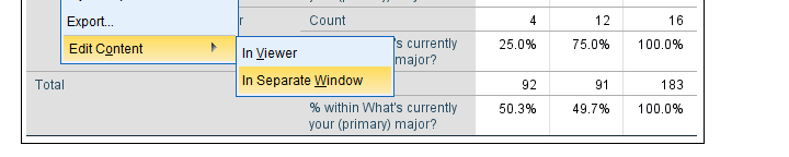
Adjusting Our Table

Since I'm not too happy with the format of my newly run table, I'll right-click it and select Edit Content In Separate Window

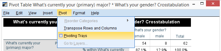
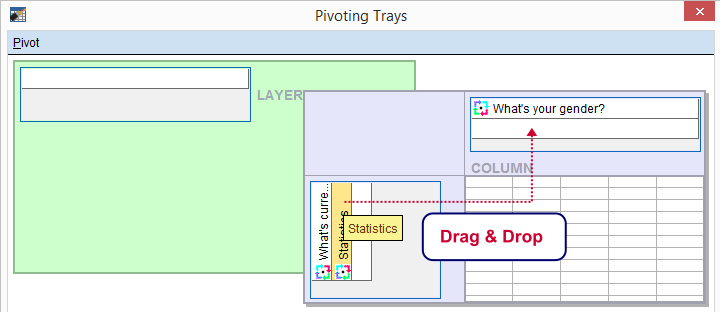
We select Pivoting Trays and then drag and drop Statistics right underneath “What's your gender?”. We'll close the pivot table editor.

Result

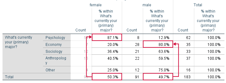
Roughly half of our sample if female. Within psychology, however, a whopping 87% is female. That is, females are highly overrepresented among psychology students. Like so, study major “says something” about gender: if I know somebody studies psychology, I know she's probably female.
The opposite pattern holds for economy students: some 80% of them are male. In short, our row percenages describe the association we established with our chi-square test.
We could quantify the strength of the association by adding Cramér’s V to our test but we'll leave that for another day.

Reporting a Chi-Square Independence Test

We report the significance test with something like “an association between gender and study major was observed, χ²(4) = 54.50, p = 0.000. Further, I suggest including our final contingency table (with frequencies and row percentages) in the report as well as it gives a lot of insight into the nature of the association.

So that's about it for now. Thanks for reading!

SPSS One Sample Chi-Square Test

SPSS one-sample chi-square test is used to test whether a single categorical variable follows a hypothesized population distribution.

SPSS One-Sample Chi-Square Test Example

A marketeer believes that 4 smartphone brands are equally attractive. He asks 43 people which brand they prefer, resulting in brands.sav. If the brands are really equally attractive, each brand should be chosen by roughly the same number of respondents. In other words, the expected frequencies under the null hypothesis are (43 cases / 4 brands =) 10.75 cases for each brand. The more the observed frequencies differ from these expected frequencies, the less likely it is that the brands really are equally attractive.

1. Quick Data Check

Before running any statistical tests, we always want to have an idea what our data basically look like. In this case we'll inspect a histogram of the preferred brand by running FREQUENCIES. We'll open the data file and create our histogram by running the syntax below. Since it's very simple, we won't bother about clicking through the menu here.

First, N = 43 means that the histogram is based on 43 cases. Since this is our sample size, we conclude that no missing values are present. SPSS also calculates a mean and standard deviation but these are not meaningful for nominal variables so we'll just ignore them. Second, the preferred brands have rather unequal frequencies, casting some doubt upon the null hypothesis of those being equal in the population.

Assumptions One-Sample Chi-Square Test

1. independent and identically distributed variables (or “independent observations”);
2. none of the expected frequencies are < 5;

The first assumption is beyond the scope of this tutorial. We'll presume it's been met by our data. Whether the assumption 2 holds is reported by SPSS whenever we run a one-sample chi-square test. However, we already saw that all expected frequencies are 10.75 for our data.

3. Run SPSS One Sample Chi-Square Test

Expected Values refers to the expected frequencies, the aforementioned 10.75 cases for each brand. We could enter these values but selecting All categories equal is a faster option and yields identical results.
Clicking Paste results in the syntax below.

4. SPSS One-Sample Chi-Square Test Output

Under Observed N we find the observed frequencies that we saw previously;
under Expected N we find the theoretically expected frequencies;They're shown as 10.8 instead of 10.75 due to rounding. All reported decimals can be seen by double-clicking the value.
for each frequency the Residual is the difference between the observed and the expected frequency and thus expresses a deviation from the null hypothesis;
the Chi-Square test statistic sort of summarizes the residuals and hence indicates the overall difference between the data and the hypothesis. The larger the chi-square value, the less the data “fit” the null hypothesis;
degrees of freedom (df) specifies which chi-square distribution applies;
Asymp. Sig. refers to the p value and is .073 in this case. If the brands are exactly equally attractive in the population, there's a 7.3% chance of finding our observed frequencies or a larger deviation from the null hypothesis. We usually reject the null hypothesis if p < .05. Since this is not the case, we conclude that the brands are equally attractive in the population.

Reporting a One-Sample Chi-Square Test

When reporting a one-sample chi-square test, we always report the observed frequencies. The expected frequencies usually follow readily from the null hypothesis so reporting them is optional. Regarding the significance test, we usually write something like “we could not demonstrate that the four brands are not equally attractive; χ²(3) = 6.95, p = .073.”