Mahalanobis Distances in SPSS – A Quick Guide

• Summary
• Mahalanobis Distances - Basic Reasoning
• Mahalanobis Distances - Formula and Properties
• Finding Mahalanobis Distances in SPSS
• Critical Values Table for Mahalanobis Distances
• Mahalanobis Distances & Missing Values

Summary

In SPSS, you can compute (squared) Mahalanobis distances as a new variable in your data file. For doing so, navigate to Analyze Regression Linear and open the “Save” subdialog as shown below.

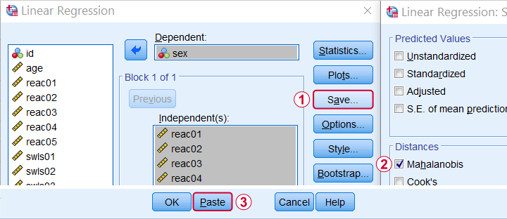
Keep in mind here that Mahalanobis distances are computed only over the independent variables. The dependent variable does not affect them unless it has any missing values. In this case, the situation becomes rather complicated as I'll cover near the end of this article.

Mahalanobis Distances - Basic Reasoning

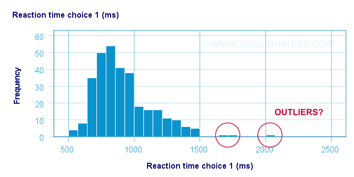
Before analyzing any data, we first need to know if they're even plausible in the first place. One aspect of doing so is checking for outliers: observations that are substantially different from the other observations. One approach here is to inspect each variable separately and the main options for doing so are

• inspecting histograms;
• inspecting boxplots or
• inspecting z-scores.

Now, when analyzing multiple variables simultaneously, a better alternative is to check for multivariate outliers: combinations of scores on 2(+) variables that are extreme or unusual. Precisely how extreme or unusual a combination of scores is, is usually quantified by their Mahalanobis distance.

The basic idea here is to add up how much each score differs from the mean while taking into account the (Pearson) correlations among the variables. So why is that a good idea? Well, let's first take a look at the scatterplot below, showing 2 positively correlated variables.

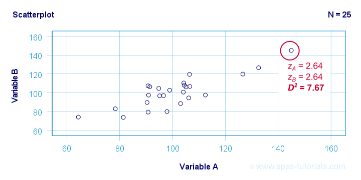
The highlighted observation has rather high z-scores on both variables. However, this makes sense: a positive correlation means that cases scoring high on one variable tend to score high on the other variable too. The (squared) Mahalanobis distance D² = 7.67 and this is well within a normal range.

So let's now compare this to the second scatterplot shown below.

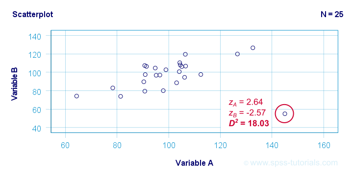
The highlighted observation has a rather high z-score on variable A but a rather low one on variable B. This is highly unusual for variables that are positively correlated. Therefore, this observation is a clear multivariate outlier because its (squared) Mahalanobis distance D² = 18.03, p < .0005. Two final points on these scatterplots are the following:

• the (univariate) z-scores fail to detect that the highlighted observation in the second scatterplot is highly unusual;
• this observation has a huge impact on the correlation between the variables and is thus an influential data point. Again, this is detected by the (squared) Mahalanobis distance but not by z-scores, histograms or even boxplots.

Mahalanobis Distances - Formula and Properties

Software for applied data analysis (including SPSS) usually computes squared Mahalanobis distances as

\(D^2_i = (\mathbf{x_i} - \mathbf{\overline{x}})'\;\mathbf{S}^{-1}\;(\mathbf{x_i} - \overline{\mathbf{x}})\)

where

• \(D^2\) denotes the squared Mahalanobis distance for case \(i\);
• \(\mathbf{x_i}\) denotes the vector of scores for case \(i\);
• \(\mathbf{\overline{x}}\) denotes the vector of means (centroid) over all cases;
• \(S\) denotes the covariance matrix over all variables.

Some basic properties are that

• Mahalanobis distances can (theoretically) range from zero to infinity;
• Mahalanobis distances are standardized: they are scale independent so they are unaffected by any linear transformations to the variables they're computed on;
• Mahalanobis distances for a single variable are equal to z-scores;
• squared Mahalanobis distances computed over k variables follow a χ²-distribution with df = k under the assumption of multivariate normality.

Finding Mahalanobis Distances in SPSS

In SPSS, you can use the linear regression dialogs to compute squared Mahalanobis distances as a new variable in your data file. For doing so, navigate to Analyze Regression Linear and open the “Save” subdialog as shown below.

Again, Mahalanobis distances are computed only over the independent variables. Although this is in line with most text books, it makes more sense to me to include the dependent variable as well. You could do so by

• adding the actual dependent variable to the independent variables and
• temporarily using an alternative dependent variable that is neither a constant, nor has any missing values.

Finally, if you've any missing values on either the dependent or any of the independent variables, things get rather complicated. I'll discuss the details at the end of this article.

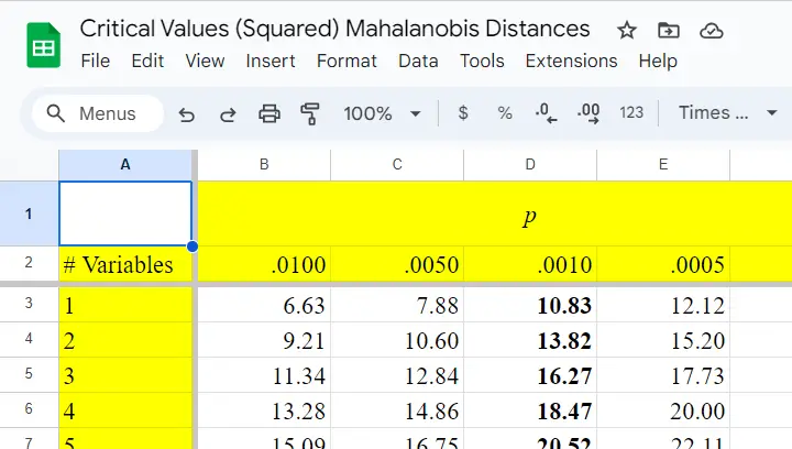
Critical Values Table for Mahalanobis Distances

After computing and inspecting (squared) Mahalanobis distances, you may wonder: how large is too large? Sadly, there's no simple rule of thumb here but most text books suggest that (squared) Mahalanobis distances for which p < .001 are suspicious for reasonable sample sizes. Since p also depends on the number of variables involved, we created a handy overview table in this Googlesheet, partly shown below.

Mahalanobis Distances & Missing Values

Missing values on either the dependent or any of the independent variables may affect Mahalanobis distances. Precisely when and how depends on which option you choose for handling missing values in the linear regression dialogs as shown below.

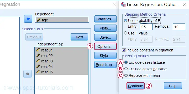
If you select listwise exclusion,

• Mahalanobis distances are computed for all cases that have zero missing values on the independent variables;
• missing values on the dependent variable may affect the Mahalanobis distances. This is because these are based on the listwise complete covariance matrix over the dependent as well as the independent variables.

If you select pairwise exclusion,

• Mahalanobis distances are computed for all cases that have zero missing values on the independent variables;
• missing values on the dependent variable do not affect the Mahalanobis distances in any way.

If you select replace with mean,

• missing values on the dependent and independent variables are replaced with the (variable) means before SPSS proceeds with any further computations;
• Mahalanobis distances are computed for all cases, regardless any missing values;
• \(D^2\) = 0 for cases having missing values on all independent variables. This makes sense because \(\mathbf{x_i} - \mathbf{\overline{x}}\) results in a vector of zeroes after replacing all missing values by means.

References

• Hair, J.F., Black, W.C., Babin, B.J. et al (2006). Multivariate Data Analysis. New Jersey: Pearson Prentice Hall.
• Warner, R.M. (2013). Applied Statistics (2nd. Edition). Thousand Oaks, CA: SAGE.
• Pituch, K.A. & Stevens, J.P. (2016). Applied Multivariate Statistics for the Social Sciences (6th. Edition). New York: Routledge.
• Field, A. (2013). Discovering Statistics with IBM SPSS Statistics. Newbury Park, CA: Sage.
• Howell, D.C. (2002). Statistical Methods for Psychology (5th ed.). Pacific Grove CA: Duxbury.
• Agresti, A. & Franklin, C. (2014). Statistics. The Art & Science of Learning from Data. Essex: Pearson Education Limited.

Mode (Statistics) – Simple Tutorial

The mode for some variable
is its value having the highest frequency.

• Mode for Continuous Variable
• Bimodal Distributions
• Finding Modes in SPSS
• Warning About Modes in Excel

Example

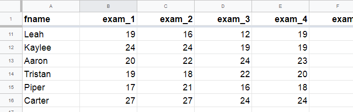
A class of 15 students take 8 exams over the academic year. The score for each exam is the number of correct answers. The data thus obtained are in this Googlesheet, partly shown below.

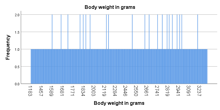
The bar chart shown below visualizes the frequency distribution for exam 1: for each score, it shows the number of students that obtained it. Scores that are absent -such as 25 and 26 points- didn't occur at all.

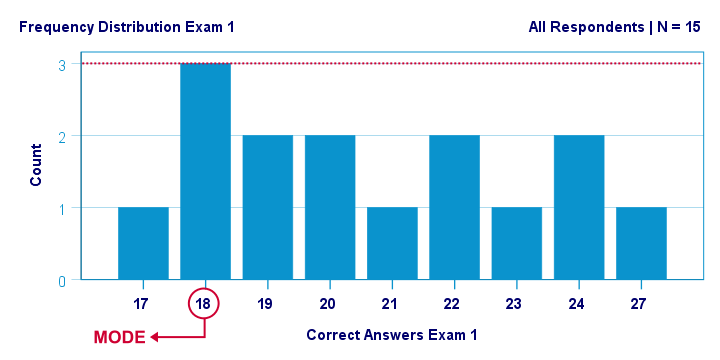
The mode for this variable is 18 points: it's the only value that occurs 3 times. All other scores occur just once or twice.

Mode for Continuous Variable

For continuous variables, the mode usually refers to the range of values
having the highest frequency. For example, we collected the body weights of N = 356 chickens in grams. The bar chart below shows the frequency distribution for this variable.

Strictly, this variable has some 15 modes and these are all weights in grams that occur twice. However, this doesn't give us any insight whatsoever. The problem is that almost every chicken has a different exact weight in grams.
The solution for this problem is inspecting fixed-width weight ranges instead of exact weights. The frequencies for these are shown in the histogram below.

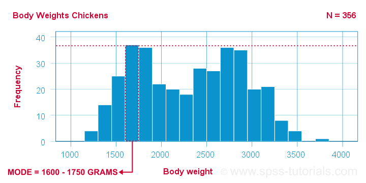
We chose a bin width of 150 grams for this chart. By doing so, the mode is the weight range from 1600 up to 1750 grams, which is observed for some 37 chickens.
Keep in mind here that the bin width is arbitrary: we could choose a different bin width and this would result in a different mode.

Bimodal Distributions

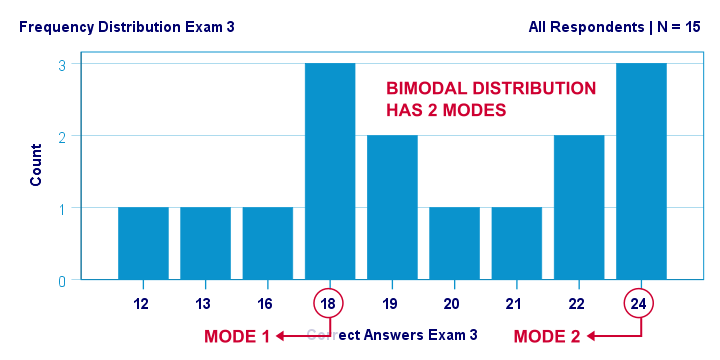
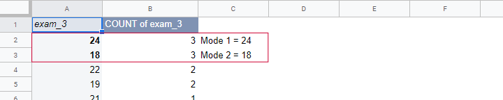
A bimodal distribution is a frequency distribution having 2 modes. An example is exam 3 in this Googlesheet, whose frequency distribution is shown below. Both 18 and 24 points occur 3 times. All other scores have lower frequencies.

For continuous variables, a bimodal distribution refers to a frequency distribution
having 2 “clear peaks” that are not necessarily equally high. Most analysts would agree that the chicken histogram we saw earlier clearly shows a bimodal distribution. In many cases, however, what constitute “clear peaks” is rather subjective and also depends on the bin width chosen.

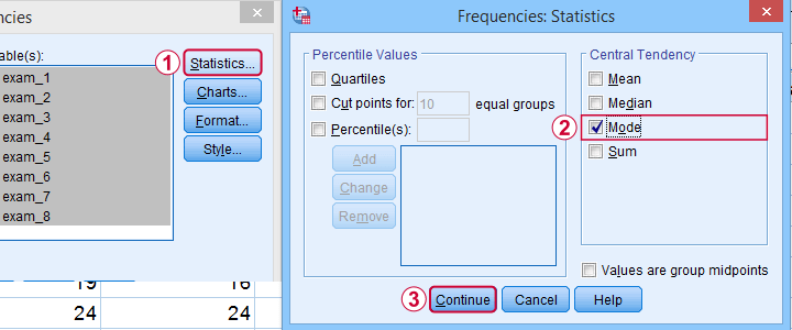
Finding Modes in SPSS

You can find modes in SPSS from Analyze Descriptive statistics Frequencies as shown below. Use exams.sav if you'd like to give it a go.

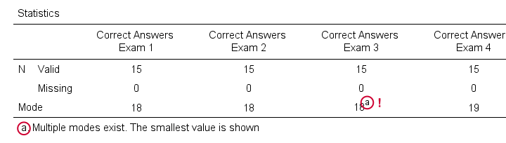
What's nice about the output -shown below- is that SPSS warns you if a variable has more than one mode. If any variables have multiple modes, the quickest way to find these is running bar charts over those variables.

Warning About Modes in Excel

For finding modes in Excel, OpenOffice and Googlesheets, type something like =MODE(A2:A16) into some cell and specify the correct range of cells over which you'd like to find the mode. This works fine if a variable has only a single mode. However, Excel does not warn you if there's multiple modes and neither do the other spreadsheet editors. So how do you know if a variable has multiple modes? Sadly, the least clumsy approach is probably creating a sorted frequency table as shown below. The need for this tedious method renders the MODE function completely worthless.

Fortunately, both SPSS and JASP do warn about multiple modes. This allows you to inspect one or many variables in a single table -an easy and fast approach.

Thanks for reading!

Median – Simple Tutorial & Examples

• Median - Simple Data Examples
• Relation Median and Mean
• Median - Strengths & Weaknesses
• Finding Medians in SPSS
• Statistical Significance for Medians - Sign Tests

The median is the middle value after sorting all values for an odd number of values. For an even number of values, it's the average of the 2 middle values after sorting all values. The examples below from this Googlesheet (read only) will make this perfectly clear.

Median - Simple Data Examples

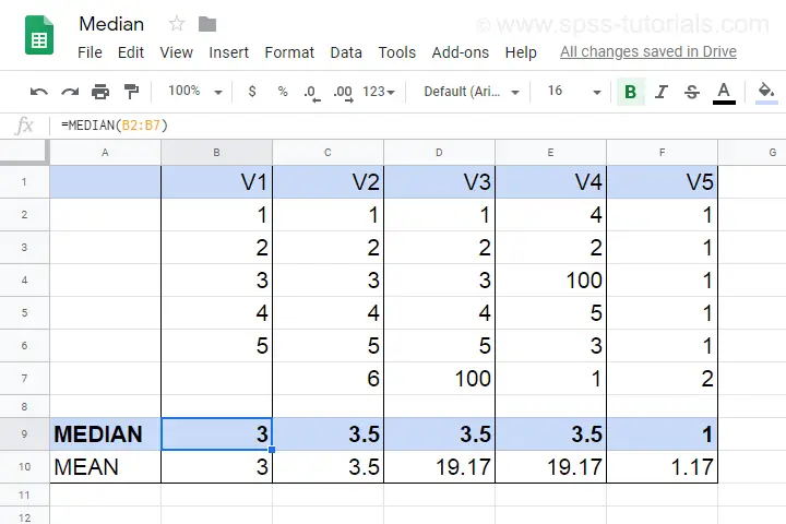
• V1 holds values 1 through 5 sorted ascendingly. The median -middle value- is 3.
• V2 holds values 1 through 6 sorted ascendingly. The median is 3.5. It is the average of the 2 middle values 3 and 4.
• V3 is V2 with 6 replaced by 100. This greatly affects the mean but the 2 middle values -and hence the median- stay the same.
• V4 holds the values of V3 in random order. The median is not the average of the 2 middle values unless we first sort them.
• V5 contains ties: the value 1 occurs 5 times. Since the values are sorted, the median is the average of the 2 middle values (1 and 1).

Note that for V2 through V4, the median is the value that separates
the 50% highest values from the 50% lowest values. This turns out to hold for most (semi)continuous variables that we find in real-world data such as

• exact monthly incomes in dollars,
• body weight in grams or
• age in days.

However, it may not hold at all for heavily tied data (such as V5) or small numbers of observations.

Relation Median and Mean

We'll discuss the pros and cons of medians versus means in a minute. Let's first see how they relate in the first place. This depends mostly on the skewness of the frequency distribution of some variable: the median is equal to the mean
for symmetrically distributed variables which implies skewness = 0. The histogram shown below illustrates this point.

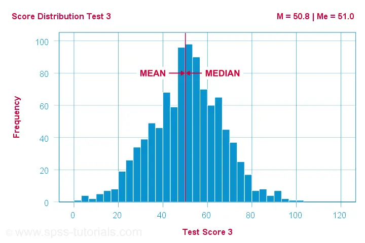
Skewness is basically zero for these 1,000 test scores. The sample mean (M) = 50.8 while the median (Me) = 51.0. The red lines indicating them on the x-axis are indistinguishable.
Different patterns occur when skewness is substantial. First off, the median is smaller than the mean
for positively skewed variables as shown below.

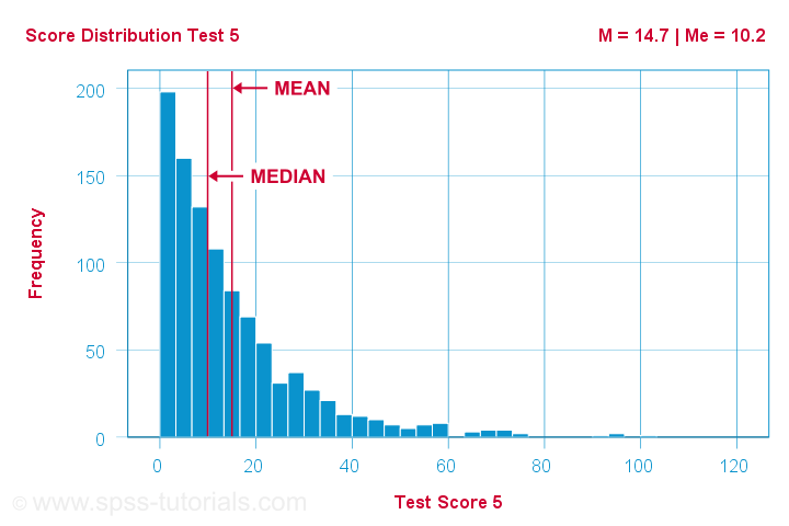
What basically happens here is that some very high scores affect the mean but not the median. We already saw this in our initial examples: changing {1,2,3,4,5,6} to {1,2,3,4,5,100} greatly affects the mean but the median is 3.5 for both variables. The histogram above shows the exact same phenomenon but it uses more realistic data.
As you can probably guess by now, the opposite also holds: the median is larger than the mean
for negatively skewed variables as illustrated by the histogram below.

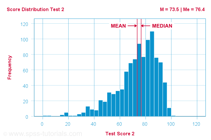
What basically happens here is that the very low scores “drag down” the mean. The median, however, is unaffected by these.

Median - Strengths & Weaknesses

Thus far, this introduction implicitly pointed out some strengths of the median compared to the mean:

• The median is not sensitive to outliers. So perhaps the mean salary for some people is high due to a single billionaire. I'd rather know the median salary in this case. This'll tell me (roughly) which salary separates the 50% lowest from the 50% highest incomes. It's a more realistic estimate of what these people tend to earn.
• Means are applicable only to quantitative variables. Medians are also suitable for ordinal variables. However, ordinal variables typically have tons of ties (values that occur more than once). For such variables, medians may be misleading as shown below.

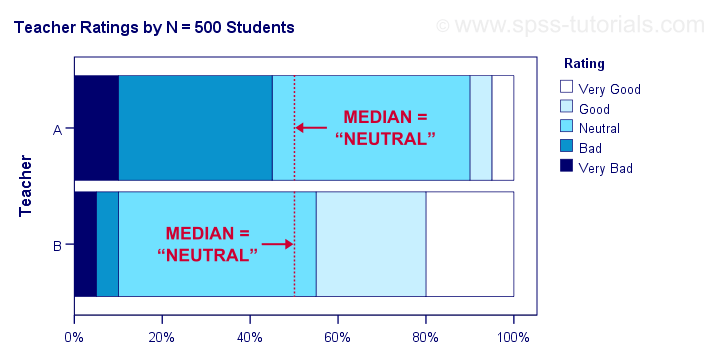
Although teacher B is rated much more favorably than teacher A, their median ratings are identical.

Apart from these strengths, medians have some weaknesses too:

• Medians are unsuitable for numeric calculations. For instance, sums can be calculated from means and sample sizes but not from medians. The difference between 2 means is easily interpretable but the difference between 2 medians hardly so.
• In the presence of ties, very different variables may have similar medians.
• The median may not actually exist. For instance, if two people have 0 and 1 children, their median is 0.5 children.
• The median is said to fluctuate more from sample to sample than the mean. That is, it is less stable and has a larger standard error.

Finding Medians in Googlesheets

Finding medians is super easy with Googlesheets. For example, typing =MEDIAN(B2:B7) into any cell results in the median of cells B2 through B7 (assuming all non empty cells contain numbers). Some more examples are shown in this Googlesheet (read only).

Finding Medians in SPSS

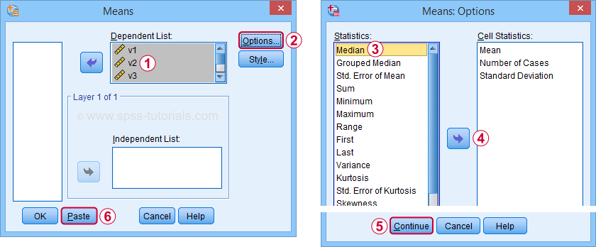
In SPSS, the best option to find medians is from Analyze Compare Means Means Use this dialog to create a table showing a wide variety of descriptive statistics including the mean, standard deviation, skewness, kurtosis and more. Optionally, these are reported for separate groups defined by “Independent List”.

An even faster option is typing and running the resulting syntax -a simple MEANS command- such as means v1 to v5
/cells count mean median. An example of the resulting table -after some adjustments- is shown below.

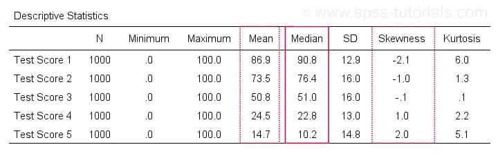
Notice the huge positive correlation between skewness and (mean - median): the median is larger than the mean insofar as a variable is more negatively (left) skewed. The opposite pattern -mean larger than median- occurs for positively (right) skewed variables. This was previously illustrated with some histograms based on the same data file as this table.

Statistical Significance for Medians - Sign Tests

Among the most popular statistical techniques are t-tests. These test if the difference between 2 means is statistically significant. But what if we want to test for medians instead of means? In this case we'll end up with one of 3 median tests, sometimes called sign tests:

• A sign test for 1 median is similar to a one sample t-test for a median: it compares the sample median to a hypothesized value.
• The sign test for independent medians is similar to an independent samples t-test or a one-way ANOVA for medians: it tests if 2 or more populations have equal medians.
• A sign test for related medians is similar to a paired samples t-test for medians: it tests if 2 variables measured on the same people or other observations have equal medians.

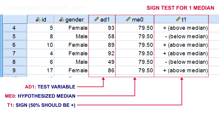
A sign test for 1 median basically works like this:

• each value smaller than the hypothesized median is replaced by a minus (-) sign;
• values larger than the hypothesized median are replaced by plus (+) signs;
• if the hypothesized median is correct, then some 50% of all signs should be plusses;
• a binomial test examines if the sample proportion of plusses is significantly different from 0.5.

The other sign tests follow the same basic reasoning. Sign tests are not very popular because ties are problematic for them and they tend to have low statistical power.

Thanks for reading!

SPSS Median Test for 2 Independent Medians

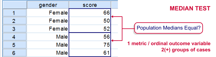
The median test for independent medians tests if two or more populations have equal medians on some variable. That is, we're comparing 2(+) groups of cases on 1 variable at a time.

Rating Car Commercials

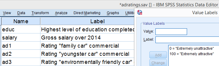
We'll demonstrate the median test on adratings.sav. This file holds data on 18 respondents who rated 3 different car commercials on attractiveness. A percent scale was used running from 0 (extremely unattractive commercial) through 100 (extremely attractive).

Median Test - Null Hypothesis

A marketeer wants to know if men rate the 3 commercials differently than women. After comparing the mean scores with a Mann-Whitney test, he also wants to know if the median scores are equal. A median test will answer the question by testing the null hypothesis that the population medians for men and women are equal for each rating variable.

Median Test - Assumptions

The median test makes only two assumptions:

• independent observations (or more precisely, independent and identically distributed variables);
• the test variable is ordinal or metric (that is, not nominal).

Quick Data Check

The adratings data don't hold any weird values or patterns. If you're analyzing any other data, make sure you always start with a data inspection. At the very least, run some histograms and check for missing values.

Median Test - Descriptives

Right, we're comparing 2 groups of cases on 3 rating variables. Let's first just take a look at the resulting 6 medians. The fastest way for doing so is running a basic MEANS command.

Result

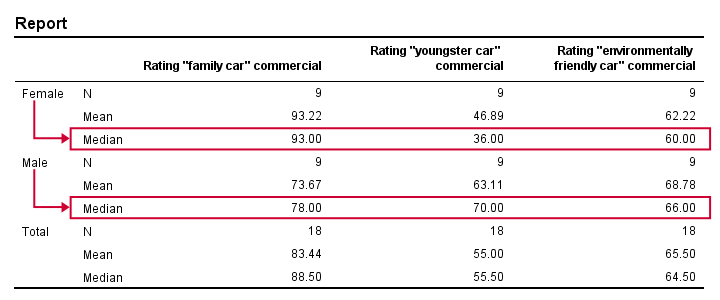
Very basically, the “family car” commercial was rated better by female respondents. Males were more attracted to the “youngster car” commercial. The “environmentally friendly car” commercial was rated roughly similarly by both genders -with regard to the medians anyway.
Now, keep in mind that this is just a small sample. If the population medians are exactly equal, then we'll probably find slightly different medians in our sample due to random sampling fluctuations. However, very different sample medians suggest that the population medians weren't equal after all. The median test tells us if equal population medians are credible, given our sample medians.

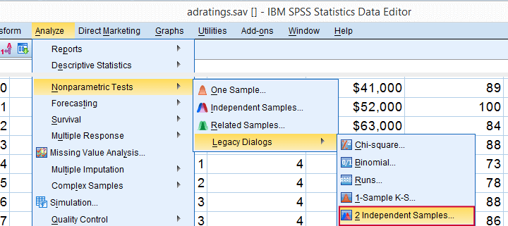
Median Test in SPSS

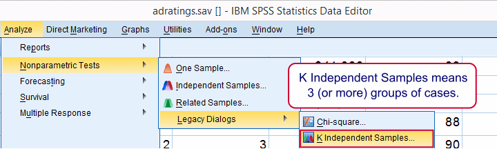
Usually, comparing 2 statistics is done with a different test than 3(+) statistics.For example, we use an independent samples t-test for 2 independent means and one-way ANOVA for 3(+) independent means. We use a paired samples t-test for 2 dependent means and repeated measures ANOVA for 3(+) dependent means. We use a McNemar test for 2 dependent proportions and a Cochran Q test for 3(+) dependent proportions. The median test is an exception because it's used for 2(+) independent medians. This is why we select K independent samples instead of 2 independent samples for comparing 2 medians.

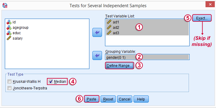
The Exact button may be absent, depending on your SPSS license. If it's present, fill it out as below.

SPSS Median Test Syntax

Completing these steps results in the syntax below (you'll have an extra line if you selected the exact test).

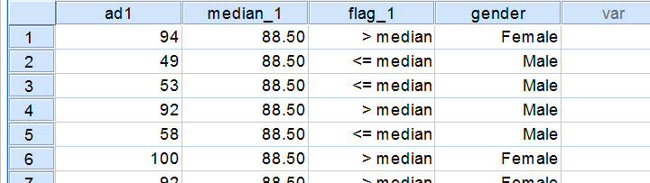
Median Test - How it Basically Works

Before inspecting our output, let's first take a look at how the test basically works for one variable.² The median test first computes a variable’s median, regardless of the groups we're comparing. Next, each case (row of data values) is flagged if its score > the pooled median. Finally, we'll see if scoring > the median is related to gender with a basic crosstab.You can pretty easily run these steps yourself with AGGREGATE, IF and CROSSTABS.

Median Test Output - Crosstabs

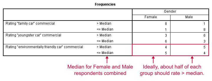
Note that these results are in line with the medians we ran earlier. The result for our “family car” commercial is particularly striking: 8 out of 9 respondents who score higher than the (pooled) median are female.

Median Test Output - Test Statistics

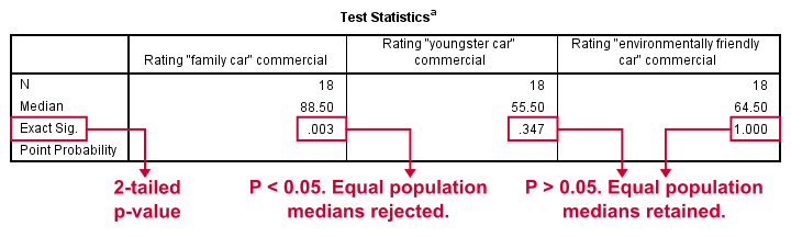
So are these normal outcomes if our population medians are equal across gender? For our first commercial, p = 0.003, indicating a chance of 3 in 1,000 of observing this outcome. Since p < 0.05, we conclude that the population medians are not equal for the “family car” commercial.
The other two commercials have p-values > 0.05 so these findings don't refute the null hypothesis of equal population medians.
So that's basically it for now. However, we would like to discuss the p-values into a little more detail for those who are interested.

Asymp. Sig.

In this example, we got exact p-values. However, when running this test on larger samples you may find “Asymp. Sig.” in your output. This is an approximate p-value based on the chi-square statistic and corresponding df (degrees of freedom). This approximation is sometimes used because the exact p-values are cumbersome to compute, especially for larger sample sizes.

Exact P-Values

So where do the exact p-values come from? How do they relate to the contingency tables we saw here? Well, the frequencies in the left upper cells follow a hypergeometric distribution.¹ Like so, the figure below shows where the second p-value of 0.347 comes from.

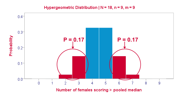
Under the null hypothesis -gender and scoring > the median are independent- the most likely outcome is 4 or 5, each with a probability around 0.33. The probability of 3 or fewer is roughly 0.17. This is our one-tailed p-value. Our two-tailed p-value takes into account the probability of 0.17 for finding a value of 6 or more because this would also contradict our null hypothesis.
The graph also illustrates why the two-tailed p-value for our third test is 1.000: the probability of 4 or fewer and 5 or more covers all possible outcomes. Regarding our first test, the probability of 1 or fewer and 8 or more is close to zero (precisely: 0.003).

Median Test with CROSSTABS

Right, so the previous figure explains how exact p-values are based on the hypergeometric distribution. This procedure is known as Fisher’s exact test and you may have seen it in SPSS CROSSTABS output when running a chi-square independence test. And -indeed- you can obtain the exact p-values for our independent medians test from CROSSTABS too. In fact, you can even compute them as a new variable in your data with compute p2 = 2* cdf.hyper(3,18,9,9).
execute. which returns 0.347, the p-value for our second commercial.

Thanks for reading!

References

1. Siegel, S. & Castellan, N.J. (1989). Nonparametric Statistics for the Behavioral Sciences (2nd ed.). Singapore: McGraw-Hill.
2. Van den Brink, W.P. & Koele, P. (2002). Statistiek, deel 3 [Statistics, part 3]. Amsterdam: Boom.

SPSS Mann-Whitney Test Tutorial

Introduction & Practice Data File

The Mann-Whitney test is an alternative for the independent samples t-test when the assumptions required by the latter aren't met by the data. The most common scenario is testing a non normally distributed outcome variable in a small sample (say, n < 25).Non normality isn't a serious issue in larger samples due to the central limit theorem.

The Mann-Whitney test is also known as the Wilcoxon test for independent samples -which shouldn't be confused with the Wilcoxon signed-ranks test for related samples.

Research Question

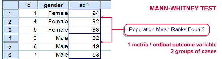
We'll use adratings.sav during this tutorial, a screenshot of which is shown above. These data contain the ratings of 3 car commercials by 18 respondents, balanced over gender and age category. Our research question is whether men and women judge our commercials similarly. For each commercial separately, our null hypothesis is: “the mean ratings of men and women are equal.”

Quick Data Check - Split Histograms

Before running any significance tests, let's first just inspect what our data look like in the first place. A great way for doing so is running some histograms. Since we're interested in differences between male and female respondents, let's split our histograms by gender. The screenshots below guide you through.

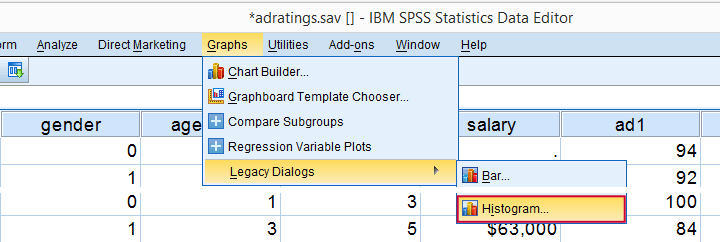
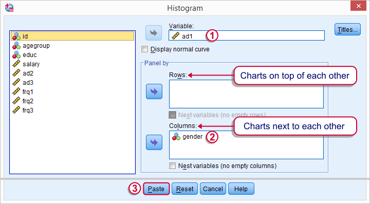
Split Histograms - Syntax

Using the menu results in the first block of syntax below. We copy-paste it twice, replace the variable name and run it.

Split Histograms - Results

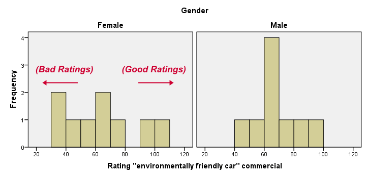
Most importantly, all results look plausible; we don't see any unusual values or patterns. Second, our outcome variables don't seem to be normally distributed and we've a total sample size of only n = 18. This argues against using a t-test for these data.
Finally, by taking a good look at the split histograms, you can already see which commercials are rated more favorably by male versus female respondents. But even if they're rated perfectly similarly by large populations of men and women, we'll still see some differences in small samples. Large sample differences, however, are unlikely if the null hypothesis -equal population means- is really true. We'll now find out if our sample differences are large enough for refuting this hypothesis.

SPSS Mann-Whitney Test - Menu

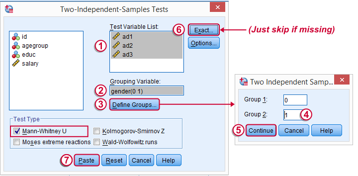
Depending on your SPSS license, you may or may not have the Exact submenu available. If you don't have it, just skip the step below.

SPSS Mann-Whitney Test - Syntax

Note: selecting Exact results in an extra line of syntax (omitted below).

SPSS Mann-Whitney Test - Output Descriptive Statistics

The Mann-Whitney test basically replaces all scores with their rank numbers: 1, 2, 3 through 18 for 18 cases. Higher scores get higher rank numbers. If our grouping variable (gender) doesn't affect our ratings, then the mean ranks should be roughly equal for men and women.

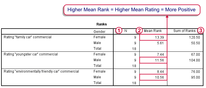
Our first commercial (“Family car”) shows the largest difference in mean ranks between male and female respondents: females seem much more enthusiastic about it. The reverse pattern -but much weaker- is observed for the other two commercials.

SPSS Mann-Whitney Test - Output Significance Tests

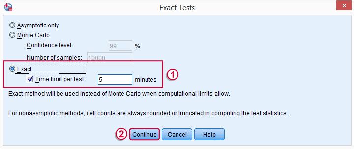
Some of the output shown below may be absent depending on your SPSS license and the sample size: for n = 40 or fewer cases, you'll always get some exact results.

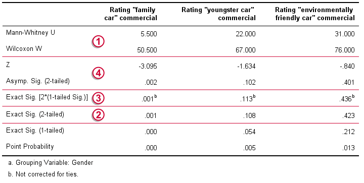
Mann-Whitney U and Wilcoxon W are our test statistics; they summarize the difference in mean rank numbers in a single number.Note that Wilcoxon W corresponds to the smallest sum of rank numbers from the previous table.
We prefer reporting Exact Sig. (2-tailed): the exact p-value corrected for ties.
Second best is Exact Sig. [2*(1-tailed Sig.)], the exact p-value but not corrected for ties.
For larger sample sizes, our test statistics are roughly normally distributed. An approximate (or “Asymptotic”) p-value is based on the standard normal distribution. The z-score and p-value reported by SPSS are calculated without applying the necessary continuity correction, resulting in some (minor) inaccuracy.

SPSS Mann-Whitney Test - Conclusions

Like we just saw, SPSS Mann-Whitney test output may include up to 3 different 2-sided p-values. Fortunately, they all lead to the same conclusion if we follow the convention of rejecting the null hypothesis if p < 0.05: Women rated the “Family Car” commercial more favorably than men (p = 0.001). The other two commercials didn't show a gender difference (p > 0.10). The p-value of 0.001 indicates a probability of 1 in 1,000: if the populations of men and women rate this commercial similarly, then we've a 1 in 1,000 chance of finding the large difference we observe in our sample. Presumably, the populations of men and women don't rate it similarly after all.

So that's about it. Thanks for reading and feel free to leave a comment below!

Measurement Levels – What and Why?

Measurement levels refer to different types of variables
that imply how to analyze them. Standard textbooks distinguish 4 such measurement levels or variable types. From low to high, these are

1. nominal variables;
2. ordinal variables;
3. interval variables;
4. ratio variables.

The “higher” the measurement level, the more information a variable holds. The simple flowchart below shows how to classify a variable.

Measurement Levels - Classical Approach

Quick Overview of Measurement Levels

Let's now take a closer look at what these variable types really mean with some examples.

Nominal Variables

A nominal variable is a variable whose
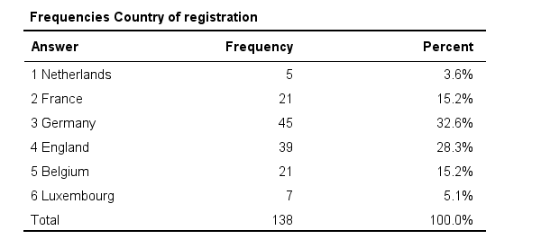
values don't have an undisputable order. So let's say we asked respondents in which country they live and the answers are

• the Netherlands;
• Belgium;
• France;
• Germany;
• Luxembourg.

So what's the correct order for these countries? Well, we could sort them alphabetically, according to their sizes or to numbers of inhabitants. Different orders make sense for a list of countries. In short, countries don't have an undisputable order and therefore “country” is a nominal variable.
Now, countries may be represented by numbers (1 = Netherlands, 2 = Belgium and so on) in SPSS or some other data format. These numbers do have an undisputable order. But country is still a nominal variable because what's represented by these numbers -countries- does not have an undisputable order.

Country -even if represented as numbers- is still a nominal variable

In a similar vein, ZIP codes -representing geographical areas which don't have a clear order- are nominal as well. But prices in dollars -representing amounts of money- obviously do have an undisputable order and hence are not nominal.

Ordinal Variables

Ordinal variables hold values that have an undisputable order
but no fixed unit of measurement. Some fixed units of measurement are meters, people, dollars or seconds. However, there's no fixed unit of measurement for a question like “how did you like your food?” with the following answer categories:

1. Bad;
2. Neutral;
3. Good.

Some may argue that Bad = 1 point, Neutral = 2 points and Good = 3 points. But that's just a wild guess. Perhaps our respondents feel Neutral represents 1.5 or 2.5 points. This is illustrated by the figure below.

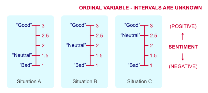Intervals between answer categories are unknown for ordinal variables.

We've no way to prove which scenario is true because just “points” are not a fixed unit of measurement. And since we don't know if Neutral represents 1.5, 2 or 2.5 points, calculations on ordinal variables are not meaningful. Less strictly though, calculations on ordinal variables are quite common under the Assumption of Equal Intervals.

Also note that monthly income measured as

1. Less than € 1000,-;
2. € 1000,- to € 2000,-;
3. € 2000,- or over.

is ordinal. Euros are a fixed unit of measurement but the answers are income categories, not numbers of Euros.

Interval Variables

Interval variables have a fixed unit of measurement
but zero does not mean “nothing”. One of the rare examples is “in which year did it happen?” Ignoring leap days, years are a fixed unit of measurement for time. However, the year zero doesn't mean “nothing” with regard to time.
As a consequence, multiplication is not meaningful for interval variables. The year 2000 isn't “twice as late” as the year 1000. The same goes for temperature in degrees Celsius: zero degrees is not “nothing” with regard to temperature. Therefore, 100 degrees is not twice as hot as 50 degrees. This argument could, however, be made for temperature in Kelvin.
We should add that these are the only 2 examples of interval variables we could think of. Interval variables are always analyzed similarly to ratio variables -which we'll turn to next. But distinguishing these as separate measurement levels -all textbooks still do- is pointless.

Ratio Variables

Ratio variables have a fixed unit of measurement
and zero really means “nothing.” An example is weight in kilos. A kilo is a fixed unit of measurement because it always represents the exact same weight. Also, zero kilos corresponds to “nothing” with regard to weight. As a consequence, multiplication is meaningful for ratio variables. In fact, we don't need more than a kitchen scale to prove that 2 times 1 kilo really is the same amount of weight as 1 time 2 kilos.

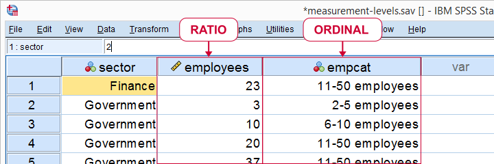Number of employees as ratio as well as ordinal variable

Some text books mention an “absolute zero point”. We rather avoid this phrasing because ratio variables may hold negative values; the balance of my bank account may be negative but it has a fixed unit of measurement -Euros in my case- and zero means “nothing”.

Classical Measurement Levels - Shortcomings

We argued that measurement levels matter because they facilitate data analysis. However, when we look at common statistical techniques, we see that

• dichotomous variables are treated differently from all other variables but classical measurement levels fail to distinguish them;
• metric variables (interval and ratio) are always treated identically;
• categorical variables (nominal and ordinal) are sometimes treated similarly and sometimes not.

Because of these reasons, we think the classification below is much more helpful.

Measurement Levels - Modern Approach

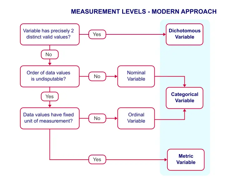
This classification distinguishes 3 main categories which we'll briefly discuss.

Dichotomous Variables

Dichotomous variables have precisely two distinct values. Typical examples are sex, owning a car or carrying HIV. It is useful to distinguish dichotomous variables as a separate measurement level because they require different analyses than other variables:

• an independent samples t-test tests if a dichotomous variable is associated with a metric variable;
• a z-test and Phi-coefficient are used to test if 2 dichotomous variables are associated;
• logistic regression predicts a dichotomous outcome variable.

Categorical Variables

Categorical variables are variables on which
calculations are not meaningful. Therefore, nominal and ordinal variables are categorical variables. They contain (usually few) answer categories. Because calculations are not meaningful, categorical variables merely define groups. We therefore analyze them with frequency distributions and bar charts.

Metric Variables

Metric variables are variables on which
calculations are meaningful. That is: interval and ratio variables are metric variables. Because calculations are allowed, we typically analyze them with descriptive statistics such as

• means;
• standard deviations;
• skewnesses.

Data Analysis - Next Steps

We just argued that

• categorical variables define groups of cases and
• we use descriptive statistics for analyzing metric variables.

Now, say we'd like to know if 2 categorical variables are associated. Then the first variable defines groups and the second variable defines groups within those groups. A table that shows just that is a contingency table as shown below. It basically holds frequency distributions within frequency distributions

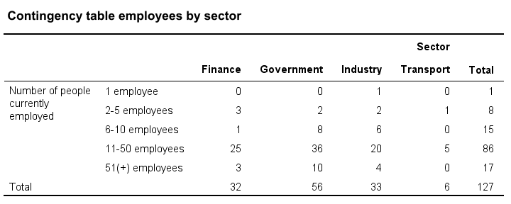
Next, we could visualize the association with a stacked bar chart. Or we may test if the association is statistically significant by running a chi-square independence test on our contingency table.

Or perhaps we'd like to know if a categorical variable and a metric variable are associated. The categorical variable defines groups. Within those groups, we'll inspect descriptive statistics over our metric variable. We thus arrive at the table as shown below.

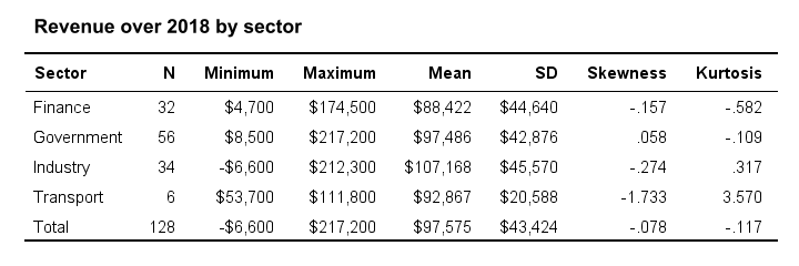
We could visualize the means as a bar chart for means by category. Or we could test if the population means differ by category with ANOVA.

So now we see how measurement levels help us choose the right analyses. For a more complete overview of analyses by measurement level, see SPSS Data Analysis - Basic Roadmap.

Thanks for reading!

McNemar Test in SPSS – Comparing 2 Related Proportions

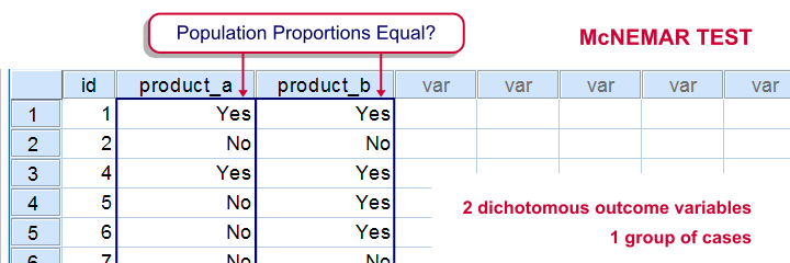
SPSS McNemar test is a procedure for testing if the proportions of two dichotomous variables are equal in some population. The two variables have been measured on the same cases.

SPSS McNemar Test Example

A marketeer wants to know whether two products are equally appealing. He asks 20 participants to try out both products and indicate whether they'd consider buying each products (“yes” or “no”). This results in product_appeal.sav. The proportion of respondents answering “yes, I'd consider buying this” indicates the level of appeal for each of the two products.
The null hypothesis is that both percentages are equal in the population.

1. Quick Data Check

Before jumping into statistical procedures, let's first just take a look at the data. A graph that basically tells the whole story for two dichotomous variables measured on the same respondents is a 3-d bar chart. The screenshots below walk you through.

We'll first navigate to Graph Legacy Dialogs 3-D Bar Click Define.

Select Number of cases and move product_a and product_b into the appropriate boxes. Clicking Paste results in the syntax below.

The most important thing we learn from this chart is that both variables are indeed dichotomous. There could have been some “Don't know/no opinion” answer category but both variables only have “Yes” and “No” answers. There are no system missing values since the bars represent (6 + 7 + 7 + 0 =) 20 valid answers which equals the number of respondents.
Second, product_b is considered by (6 + 7 =) 13 respondents and thus seems more appealing than product_a (considered by 7 respondents). Third, all of the respondents who consider product_a consider product_b as well but not reversely. This causes the variables to be positively correlated and asks for a close look at the nature of both products.

2. Assumptions McNemar Test

The results from the McNemar test rely on just one assumption:

• independent and identically distributed variables (or, less precisely, “independent observations”);

3. Run SPSS McNemar Test

We'll navigate to Analyze Nonparametric Tests Legacy Dialogs 2 Related Samples....

We select both product variables and move them into the Test Pairs box.
Under Options, we'll select Descriptives.
We only select McNemar under Test Type
Clicking Paste results in the syntax below.

4. SPSS McNemar Test Output

The first table (Descriptive Statistics) confirms that there are no missing values. We already saw this in our chart as well.If there are missing values, these descriptives may be misleading. This is because they use pairwise deletion of missing values while the significance test (necessarily) uses listwise deletion of missing values. Therefore, the descriptives may use different data than the actual test. This deficiency can be circumvented by (manually) FILTERING out all incomplete cases before running the McNemar test.
Note that SPSS reports means rather than proportions. However, if your answer categories are coded 0 (for “absent”) and 1 (for “present”) the means coincide with the proportions.We suggest you RECODE your values if this is not the case. The proportions are (exactly) .35 and .65. The difference is thus -.3 where we expected 0 (equal proportions).

The second table (Test Statistics) shows that the p-value is .031. If the two proportions are equal in the population, there's only a 3.1% chance of finding the difference we observed in our sample. Usually, if p < .05, we reject the null hypothesis. We therefore conclude that the appeal of both products is not equal.
Note that the p-value is two-sided. It consists of a .0155 chance of finding a difference smaller than (or equal to) -.3 and another .0155 chance of finding a difference larger than (or equal to) .3.

5. Reporting the McNemar Test Result

In any case, we report the two proportions and the sample size on which they were based, probably in the style of the descriptives table we saw earlier. For reporting the significance test we can write something like “A McNemar test showed that the two proportions were different, p = .031 (2 sided).”