SPSS SET – Quick Tutorial
Why should you learn anything about your SPSS settings? Well, doing so allows you to
- create better output with less effort;
- speed up a huge variety of tasks;
- accomplish tasks that are otherwise impossible.
So which settings are interesting to learn about? The table below presents our top 10.
Top 10 Most Useful SPSS Settings
| SETTING | OPTIONS | DESCRIPTION |
|---|---|---|
| TNUMBERS | BOTH / LABELS / VALUES | How to show values in pivot tables |
| TVARS | BOTH / LABELS / NAMES | How to show variables in pivot tables |
| OVARS | BOTH / LABELS / NAMES | How to show variables in output viewer outline |
| TLOOK | (path to .stt file) / NONE | Tablelook file: styling for pivot tables |
| SIGLESS | ON / OFF | Whether to display small significance levels as < 0.001 in tables |
| CTEMPLATE | (path to .sgt file) / NONE | Chart template file: styling for charts |
| LOCALE | (locale) / OSLOCALE | Country and character set |
| SEED | (chosen integer) / RANDOM | Random seed used if RNG = MC |
| PRINTBACK | NONE / LISTING | Whether to print syntax to output viewer |
| ODISPLAY | MODELVIEWER / TABLES | Whether to use model viewer for some output |
Background & Googlesheet for All Settings
The vast majority of settings can be adjusted by navigating to
![]() as shown below.
as shown below.
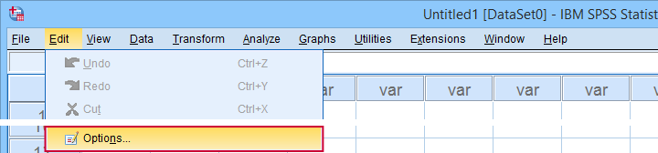
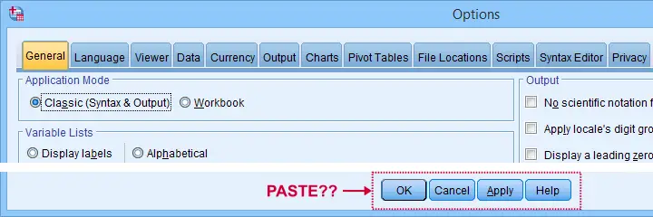
Sadly, the options dialog is a bit of a labyrinth and finding your way here can be time consuming. Another major stupidity is that there's no Paste button here either.
For these reasons, using SPSS syntax is a much better option for adjusting your settings. But where to start? Well, first off, we created an overview of all settings in this Googlesheet, partly shown below.
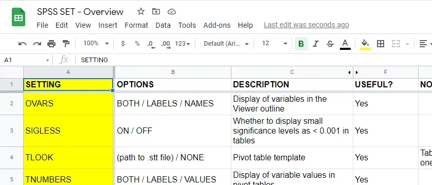
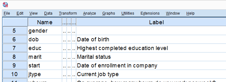
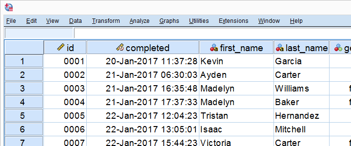
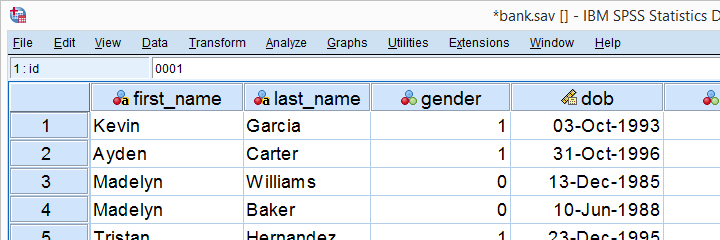
Note that Column F suggests if we think some setting is useful. The remainder of this tutorial demonstrates the 10 most useful settings, ordered from most to least important. All examples use bank-clean.sav, partly shown below.
SET TNUMBERS - Table Numbers
TNUMBERS controls how values are shown in output tables. The syntax below presents a quick demo.
set tnumbers both.
*Run minimal frequency table.
frequencies marit.
*Show only value labels in all succeeding tables.
set tnumbers labels.
*Run minimal frequency table.
frequencies marit.
Result
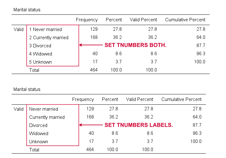
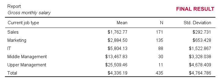
Reporting values and value labels is the recommended setting for screening data. However, for creating “clean” tables to include in your final report, you probably want to show only value labels.
SET TVARS - Table Variables
TVARS controls how variables are shown in output tables. For a quick demo, try the syntax below.
set tvars both.
*Run minimal descriptives table.
descriptives q1 to q3.
*Show only variable labels in succeeding output tables.
set tvars labels.
*Run minimal descriptives table.
descriptives q1 to q3.
Result
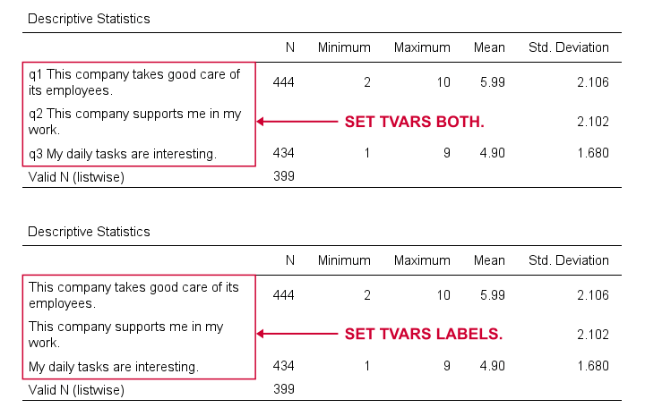
For screening data, showing both variable names and labels is often the way to go. For creating reporting tables, however, we recommend showing only variable labels.
SET OVARS - Outline Variables
OVARS controls how variables are shown in the output outline. The syntax below gives a quick demo.
set ovars both.
*Frequency tables & barcharts.
frequencies q1 to q3
/barchart.
*Show only variable names in viewer outline.
set ovars names.
*Frequency tables & barcharts.
frequencies q1 to q3
/barchart.
Result
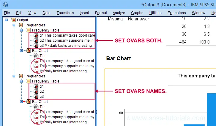
Note that the OVARS setting ignores the bar charts created with the frequency tables. The same goes for histograms. We believe this to be a tiny -but sometimes annoying- bug in SPSS.
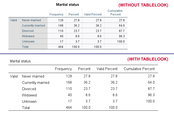
SET TLOOK - Tablelook
Tablelooks or .stt files are plain text files containing styling for tables such as fonts, background colors and borders. The syntax demo below requires that clean-11pt.stt is located in a folder d:/templates on your computer.
set tlook none.
*Run minimal frequency table.
frequencies marit.
*Set nicer tablelook.
set tlook 'd:/templates/clean-11pt.stt'.
*Run minimal frequency table.
frequencies marit.
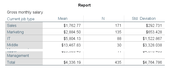
Result
Notes
- You can also apply tablelooks to existing tables by using the menu or (faster) OUTPUT MODIFY.
- Sadly, the TLOOK setting ignores the CD command: you always need to specify both the folder and the file name...
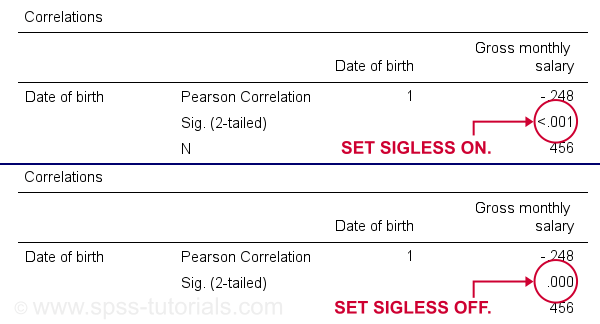
SET SIGLESS - Significance Less Than...
SIGLESS (introduced in SPSS 27) controls how small significance levels are shown in output tables. We believe there's a bug regarding this setting: the syntax below ignores it unless you run each line separately.
set sigless on.
*Run minimal correlation matrix.
correlations dob salary.
*Show small p-values as .000.
set sigless off.
*Run minimal correlation matrix.
correlations dob salary.
Result
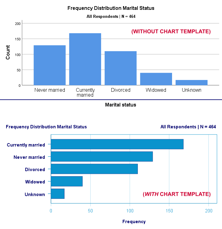
SET CTEMPLATE - Chart Template
Chart templates or .sgt files are plain text files containing styling for charts such as colors, sizes and layout. The quick demo below requires that barchart-freq-dsort-en-h360.sgt is located in a folder d:/templates on your computer.
set ctemplate none.
*Minimal bar chart frequencies.
GRAPH
/BAR(SIMPLE)=COUNT BY marit
/TITLE='Frequency Distribution Marital Status'
/SUBTITLE='All Respondents | N = 464'.
*Set chart template for bar charts.
set ctemplate 'd:/templates/barchart-freq-dsort-en-h360.sgt'.
*Minimal bar chart frequencies.
GRAPH
/BAR(SIMPLE)=COUNT BY marit
/TITLE='Frequency Distribution Marital Status'
/SUBTITLE='All Respondents | N = 464'.
Result
Notes
- After creating the charts you need, you probably want to set your CTEMPLATE back to NONE.
- Some commands (GRAPH, GGRAPH) have a /TEMPLATE subcommand for applying chart templates but this doesn't work properly.
- You can also apply chart templates to existing charts from the menu or (faster) OUTPUT MODIFY.
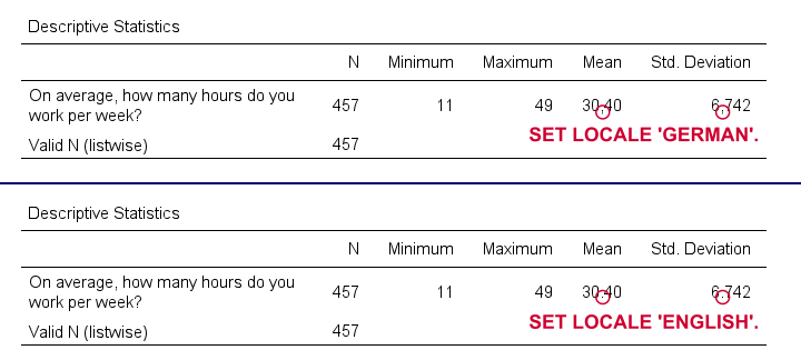
SET LOCALE
In recent SPSS versions, LOCALE is mainly used for specifying which decimal separator to use. It may also affect which character encoding SPSS uses but only if UNICODE = OFF (rarely used anymore).
set locale 'german'.
*Run minimal descriptives table.
descriptives whours.
*Set locale to German (dot as decimal separator).
set locale 'english'.
*Run minimal descriptives table.
descriptives whours.
Result
Quick note: I often prefer to use the DOT and COMMA formats for choosing which decimal separator is used. Doing so also makes converting string to numeric variables independent of your settings as discussed in SPSS Convert String to Numeric Variable. The syntax below, however, simply replicates the previous example using this alternative method.
formats whours(dot2).
*Run minimal descriptives table.
descriptives whours.
*Set format whours to comma (dot as decimal separator).
formats whours (comma2).
*Run minimal descriptives table.
descriptives whours.
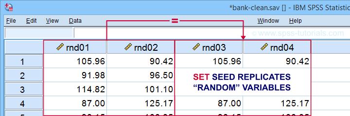
SET SEED - Random Seed
Setting a random seed allows you to exactly replicate anything random in SPSS: computing random variables or drawing random samples. The example below computes two normally distributed random variables and then exactly replicates both.
set seed 1.
*Compute two "random" variables.
compute rnd01 = rv.normal(100,15).
compute rnd02 = rv.normal(100,15).
execute.
*Reset random seed to 1 (assuming RNG = MC).
set seed 1.
*Replicate previous "random" variables.
compute rnd03 = rv.normal(100,15).
compute rnd04 = rv.normal(100,15).
execute.
Result
Minor note: SET SEED only takes effect if RNG = MC (default). You need to use SET MTINDEX if RNG = MT but I don't think anybody ever uses that.
SET PRINTBACK
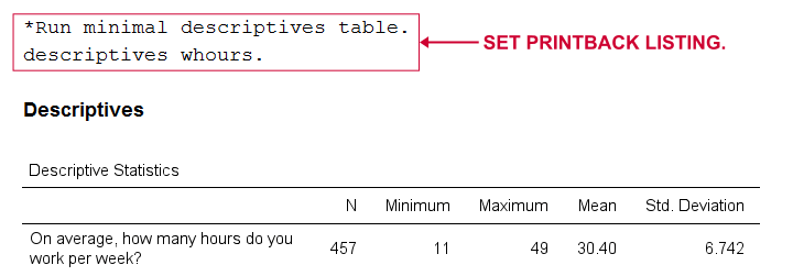
PRINTBACK tells SPSS whether to print the syntax you run (either from a syntax window or the menu) into your output window. Doing so may come in handy if you export all output to a single .pdf or WORD file.
set printback listing.
*Run minimal descriptives table.
descriptives whours.
*Don't print syntax into output viewer.
set printback none.
*Run minimal descriptives table.
descriptives whours.
Result
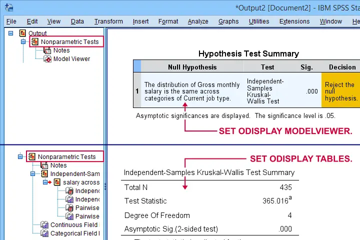
SET ODISPLAY - Output Display
For GENLINMIXED and NPTESTS, two output formats are available:
- the dreadful “model viewer” object or
- normal output (pivot) tables.
The syntax below creates both formats for a basic Kruskal-Wallis test.
set odisplay modelviewer.
*Kruskal-Wallis test.
NPTESTS
/INDEPENDENT TEST (salary) GROUP (jtype) KRUSKAL_WALLIS(COMPARE=PAIRWISE)
/MISSING SCOPE=ANALYSIS USERMISSING=EXCLUDE
/CRITERIA ALPHA=0.05 CILEVEL=95.
*Create pivot tables for NPTESTS (recommended).
set odisplay tables.
*Kruskal-Wallis test.
NPTESTS
/INDEPENDENT TEST (salary) GROUP (jtype) KRUSKAL_WALLIS(COMPARE=PAIRWISE)
/MISSING SCOPE=ANALYSIS USERMISSING=EXCLUDE
/CRITERIA ALPHA=0.05 CILEVEL=95.
Result
Note: I usually prefer a completely different command for the Kruskal-Wallis test as discussed in How to Run a Kruskal-Wallis Test in SPSS? This method does not include pairwise comparisons but I'm not a big fan of those anyway.
Related Commands - SHOW, PRESERVE & RESTORE
Before closing off, I should point out that you can use SHOW for looking up settings. Like so, SHOW ALL. shows all settings. These include some that you can't set with SET and some that you can't change at all.
Last but not least, you can undo changes in settings by preceding SET with PRESERVE and succeeding it with RESTORE. I find these commands mostly useful for building SPSS tools that change somebody else’s settings.
Right, I hope you found this tutorial helpful. Let me know if you (dis)agree and/or if I missed anything by throwing a quick comment below. Other than that:
Thanks for reading!
SPSS FILTER – Quick & Simple Tutorial
SPSS FILTER temporarily excludes a selection of cases
from all data analyses.
For excluding cases from data editing, use DO IF or IF instead.
Quick Overview Contents
- SPSS Filtering Basics
- Example 1 - Exclude Cases with Many Missing Values
- Example 2 - Filter on 2 Variables
- Example 3 - Filter without Filter Variable
- Tip - Commands with Built-In Filters
- Warning - Data Editing with Filter
SPSS FILTER - Example Data
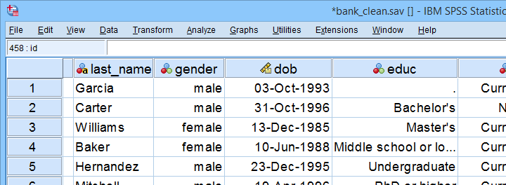
I'll use bank_clean.sav -partly shown below- for all examples in this tutorial. This file contains the data from a small bank employee survey. Feel free to download these data and rerun the examples yourself.

SPSS Filtering Basics
Filtering in SPSS usually involves 4 steps:
- create a filter variable;
- activate the filter variable;
- run one or many analyses -such as correlations, ANOVA or a chi-square test- with the filter variable in effect;
- deactivate the filter variable.
In theory, any variable can be used as a filter variable. After activating it, cases with
- zeroes,
- user missing values or
- system missing values
on the filter variable are excluded from all analyses until you deactivate the filter. For the sake of clarity, I recommend you only use filter variables containing 0 or 1 for each case. Enough theory. Let's put things into practice.
Example 1 - Exclude Cases with Many Missing Values
At the end of our data, we find 9 rating scales: q1 to q9. Perhaps we'd like to run a factor analysis on them or use them as predictors in regression analysis. In any case, we may want to exclude cases having many missing values on these variables. We'll first just count them by running the syntax below.
compute mis_1 = nmiss(q1 to q9).
*Apply variable label.
variable labels mis_1 'Number of missings on q1 to q9'.
*Check frequencies.
frequencies mis_1.
Result
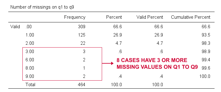
Based on this frequency distribution, we decided to exclude the 8 cases having 3 or more missing values on q1 to q9. We'll create our filter variable with a simple RECODE as shown below.
recode mis_1 (lo thru 2 = 1)(else = 0) into filt_1.
*Apply variable label.
variable labels filt_1 'Filter out cases with 3 or more missings on q1 to q9'.
*Activate filter variable.
filter by filt_1.
*Reinspect numbers of missings over q1 to q9.
frequencies mis_1.
Result
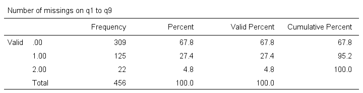
Note that SPSS now reports 456 instead of 464 cases. The 8 cases with 3 or more missing values are still in our data but they are excluded from all analyses. We can see why in data view as shown below.
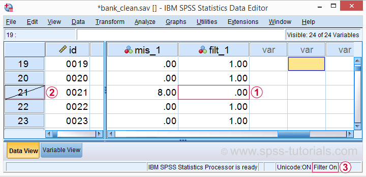
 Case 21 has 8 missing values on q1 to q9 and we recoded this into zero on our filter variable.
 The strikethrough its $casenum shows that case 21 is currently filtered out.
 The status bar confirms that a filter variable is in effect.
Finally, let's deactivate our filter by simply running
FILTER OFF.
We'll leave our filter variable filt_1 in the data. It won't bother us in any way.
The status bar confirms that a filter variable is in effect.
Finally, let's deactivate our filter by simply running
FILTER OFF.
We'll leave our filter variable filt_1 in the data. It won't bother us in any way.
Example 2 - Filter on 2 Variables
For some other analysis, we'd like to use only female respondents working in sales or marketing. A good starting point is running a very simple contingency table as shown below.
set tnumbers both.
*Show frequencies for job type per gender.
crosstabs gender by jtype.
Result
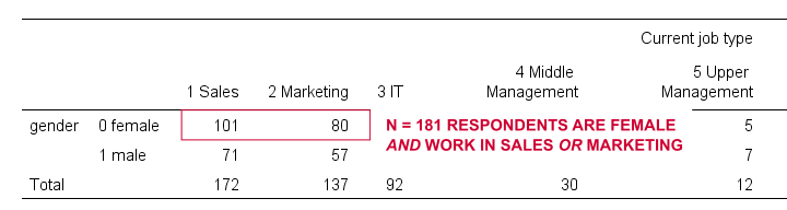
As our table shows, we've 181 female respondents working in either sales or marketing. We'll now create a new filter variable holding only zeroes. We'll then set it to 1 for our case selection with a simple IF command.
compute filt_2 = 0.
*Set filter to 1 for females in job types 1 and 2.
if(gender = 0 & jtype <= 2) filt_2 = 1.
*Apply variable label.
variable labels filt_2 'Filter in females working in sales and marketing'.
*Activate filter.
filter by filt_2.
*Confirm filter working properly.
crosstabs gender by jtype.
Rerunning our contingency table (not shown) confirms that SPSS now reports only 181 female cases working in marketing or sales. Also note that we now have 2 filter variables in our data and that's just fine but only 1 filter variable can be active at any time. Ok. Let's deactivate our new filter variable as well with FILTER OFF.
Example 3 - Filter without Filter Variable
Experienced SPSS users may know that
- TEMPORARY can “undo” some data editing that follow it and
- SELECT IF permanently deletes cases from your data.
By combining them you can circumvent the need for creating a filter variable but for 1 analysis at the time only. The example below shows just that: the first CROSSTABS is limited to a selection of cases but also rolls back our case deletion. The second CROSSTABS therefore includes all cases again.
temporary.
*Delete cases unless gender = 1 & jtype = 3.
select if (gender = 1 & jtype = 3).
*Crosstabs includes only males in IT and rolls back case selection.
crosstabs gender by jtype.
*Crosstabs includes all cases again.
crosstabs gender by jtype.
Tip - Commands with Built-In Filters
Something else you may want to know is that some commands have a built-in filter. These are
- REGRESSION,
- LOGISTIC REGRESSION,
- FACTOR and
- DISCRIMINANT.
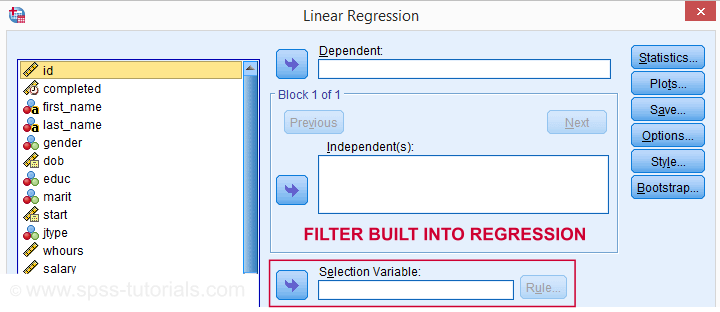
The dialog suggests you can filter cases -for this command only- based on just 1 variable. I suspect you can enter more complex conditions on the resulting /SELECT subcommand as well. I haven't tried it.
In any case, I think these built-in filters can be very handy and it kinda puzzles me they're only limited to the 4 aforementioned commands.
Warning - Data Editing with Filter
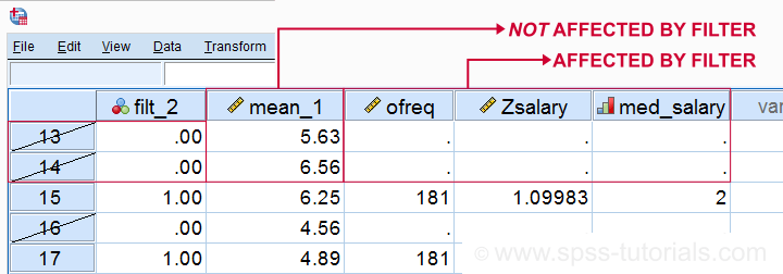
Most data editing in SPSS is unaffected by filtering. For example, computing means over variables -as shown below- affects all cases, regardless of whatever filter is active. We therefore need DO IF or IF to restrict this transformation to a selection of cases. However, an active filter does affect functions over cases. Some examples that we'll demonstrate below are
- adding a case count with AGGREGATE;
- computing z-scores for one or many variables;
- adding ranks, or percentiles with RANK.
SPSS Data Editing Affected by Filter Examples
filter by filt_2.
*Not affected by filter: add mean over q1 to q9 to data.
compute mean_1 = mean(q1 to q9).
execute.
*Affected by filter: add case count to data.
aggregate outfile * mode addvariables
/ofreq = n.
*Affected by filter: add z-scores salary to data..
descriptives salary
/save.
*Affected by filter: add median groups salary to data.
rank salary
/ntiles(2) into med_salary.
Result
Right. So that's pretty much all about filtering in SPSS. I hope you found this tutorial helpful and
Thanks for reading!
SPSS IF – A Quick Tutorial
In SPSS, IF computes a new or existing variable
for a selection of cases.
For analyzing a selection of cases, use FILTER or SELECT IF instead.
- Example 1 - Flag Cases Based on Date Function
- Example 2 - Replace Range of Values by Function
- Example 3 - Compute Variable Differently Based on Gender
- SPSS IF Versus DO IF
- SPSS IF Versus RECODE
Data File Used for Examples
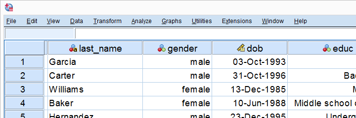
All examples use bank.sav, a short survey of bank employees. Part of the data are shown below. For getting the most out of this tutorial, we recommend you download the file and try the examples for yourself.
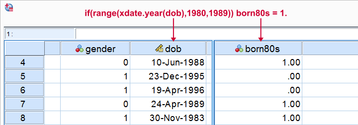
Example 1 - Flag Cases Based on Date Function
Let's flag all respondents born during the 80’s. The syntax below first computes our flag variable -born80s- as a column of zeroes. We then set it to one if the year -extracted from the date of birth- is in the RANGE 1980 through 1989.
compute born80s = 0.
*Set value to 1 if respondent born between 1980 and 1989.
if(range(xdate.year(dob),1980,1989)) born80s = 1.
execute.
*Optionally: add value labels.
add value labels born80s 0 'Not born during 80s' 1 'Born during 80s'.
Result
Example 2 - Replace Range of Values by Function
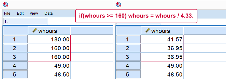
Next, if we'd run a histogram on weekly working hours -whours- we'd see values of 160 hours and over. However, weeks only hold (24 * 7 =) 168 hours. Even Kim Jong Un wouldn't claim he works 160 hours per week!
We assume these respondents filled out their monthly -rather than weekly- working hours. On average, months hold (52 / 12 =) 4.33 weeks. So we'll divide weekly hours by 4.33 but only for cases scoring 160 or over.
sort cases by whours (d).
*Divide 160 or more hours by 4.33 (average weeks per month).
if(whours >= 160) whours = whours / 4.33.
execute.
Result
Note
We could have done this correction with RECODE as well: RECODE whours (160 = 36.95)(180 = 41.57). Note, however, that RECODE becomes tedious insofar as we must correct more distinct values. It works reasonably for this variable but IF works great for all variables.
Example 3 - Compute Variable Differently Based on Gender
We'll now flag cases who work fulltime. However, “fulltime” means 40 hours for male employees and 36 hours for female employees. So we need to use different formulas based on gender. The IF command below does just that.
compute fulltime = 0.
*Set fulltime to 1 if whours >= 36 for females or whours >= 40 for males.
if(gender = 0 & whours >= 36) fulltime = 1.
if(gender = 1 & whours >= 40) fulltime = 1.
*Optionally, add value labels.
add value labels fulltime 0 'Not working fulltime' 1 'Working fulltime'.
*Quick check.
means whours by gender by fulltime
/cells min max mean stddev.
Result
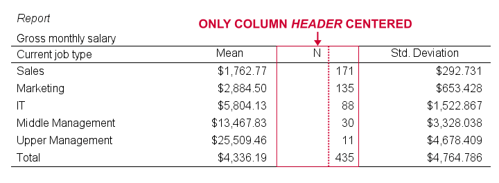
Our syntax ends with a MEANS table showing minima, maxima, means and standard deviations per gender per group. This table -shown below- is a nice way to check the results.
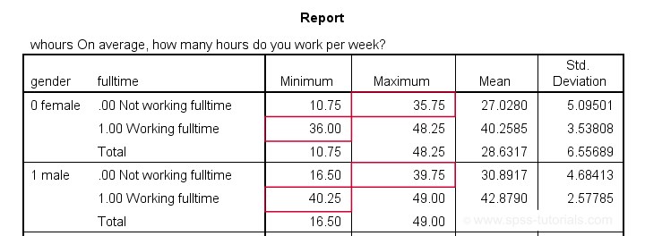
The maximum for females not working fulltime is below 36. The minimum for females working fulltime is 36. And so on.
SPSS IF Versus DO IF
Some SPSS users may be familiar with DO IF. The main differences between DO IF and IF are that
- IF is a single line command while DO IF requires at least 3 lines: DO IF, some transformation(s) and END IF.
- IF is a conditional COMPUTE command whereas DO IF can affect other transformations -such as RECODE or COUNT- as well.
- If cases meet more than 1 condition, the first condition prevails when using DO IF - ELSE IF. If you use multiple IF commands instead, the last condition met by each case takes effect. The syntax below sketches this idea.
DO IF - ELSE IF Versus Multiple IF Commands
do if(condition_1).
result_1.
else if(condition_2). /*excludes cases meeting condition_1.
result_2.
end if.
*IF: respondents meeting both conditions get result_2.
if(condition_1) result_1.
if(condition_2) result_2. /*includes cases meeting condition_1.
SPSS IF Versus RECODE
In many cases, RECODE is an easier alternative for IF. However, RECODE has more limitations too.
First off, RECODE only replaces (ranges of) constants -such as 0, 99 or system missing values- by other constants. So something like
recode overall (sysmis = q1).
is not possible -q1 is a variable, not a constant- but
if(sysmis(overall)) overall = q1.
works fine. You can't RECODE a function -mean, sum or whatever- into anything nor recode anything into a function. You'll need IF for doing so.
Second, RECODE can only set values based on a single variable. This is the reason why
you can't recode 2 variables into one
but you can use an IF condition involving multiple variables:
if(gender = 0 & whours >= 36) fulltime = 1.
is perfectly possible.
You can get around this limitation by combining RECODE with DO IF, however. Like so, our last example shows a different route to flag fulltime working males and females using different criteria.
Example 4 - Compute Variable Differently Based on Gender II
recode whours (40 thru hi = 1)(else = 0) into fulltime2.
*Apply different recode for female respondents.
do if(gender = 0).
recode whours (36 thru hi = 1)(else = 0) into fulltime2.
end if.
*Optionally, add value labels.
add value labels fulltime2 0 'Not working fulltime' 1 'Working fulltime'.
*Quick check.
means whours by gender by fulltime2
/cells min max mean stddev.
Final Notes
This tutorial presented a brief discussion of the IF command with a couple of examples. I hope you found them helpful. If I missed anything essential, please throw me a comment below.
Thanks for reading!
SPSS SELECT IF – Tutorial & Examples
Quick Overview Contents
In SPSS, SELECT IF permanently removes
a selection of cases (rows) from your data.
- Example 1 - Selection for 1 Variable
- Example 2 - Selection for 2 Variables
- Example 3 - Selection for (Non) Missing Values
- Tip 1 - Inspect Selection Before Deletion
- Tip 2 - Use TEMPORARY
Summary
SELECT IF in SPSS basically means “delete all cases that don't satisfy one or more conditions”. Like so, select if(gender = 'female'). permanently deletes all cases whose gender is not female. Let's now walk through some real world examples using bank_clean.sav, partly shown below.
Example 1 - Selection for 1 Variable
Let's first delete all cases who don't have at least a Bachelor's degree. The syntax below:
- inspects the frequency distribution for education level;
- deletes unneeded cases;
- inspects the results.
set tnumbers both.
*Run minimal frequencies table.
frequencies educ.
*Select cases with a Bachelor's degree or higher. Delete all other cases.
select if(educ >= 4).
*Reinspect frequencies.
frequencies educ.
Result
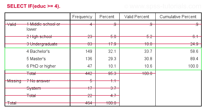
As we see, our data now only contain cases having a Bachelor's, Master's or PhD degree. Importantly, cases having
on education level have been removed from the data as well.
Example 2 - Selection for 2 Variables
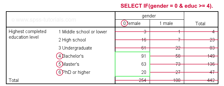
The syntax below selects cases based on gender and education level: we'll keep only female respondents having at least a Bachelor's degree in our data.
crosstabs educ by gender.
*Select females having a Bachelor's degree or higher.
select if(gender = 0 & educ >= 4).
*Reinspect contingency table.
crosstabs educ by gender.
Result
Example 3 - Selection for (Non) Missing Values
Selections based on (non) missing values are straightforward if you master SPSS Missing Values Functions. For example, the syntax below shows 2 options for deleting cases having fewer than 7 valid values on the last 10 variables (overall to q9).
select if(nvalid(overall to q9) >= 7)./*At least 7 valid values or at most 3 missings.
execute.
*Alternative way, exact same result.
select if(nmiss(overall to q9) < 4)./*Fewer than 4 missings or more than 6 valid values.
execute.
Tip 1 - Inspect Selection Before Deletion
Before deleting cases, I sometimes want to have a quick look at them. A good way for doing so is creating a FILTER variable. The syntax below shows the right way for doing so.
compute filt_1 = 0.
*Set filter variable to 1 for cases we want to keep in data.
if(nvalid(overall to q9) >= 7) filt_1 = 1.
*Move unselected cases to bottom of dataset.
sort cases by filt_1 (d).
*Scroll to bottom of dataset now. Note that cases 459 - 464 will be deleted because they have 0 on filt_1.
*If selection as desired, delete other cases.
select if(filt_1).
execute.
Quick note: select if(filt_1). is a shorthand for select if(filt_1 <> 0). and deletes cases having either a zero or a missing value on filt_1.
Result
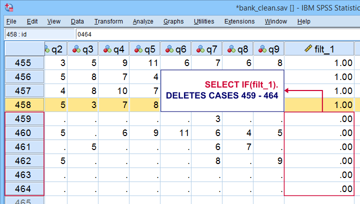 Cases that will be deleted are at the bottom of our data. We also readily see we'll have 458 cases left after doing so.
Tip 2 - Use TEMPORARY
A final tip I want to mention is combining SELECT IF with TEMPORARY. By doing so, SELECT IF only applies to the first procedure that follows it. For a quick example, compare the results of the first and second FREQUENCIES commands below.
temporary.
*Select only female cases.
select if(gender = 0).
*Any procedure now uses only female cases. This also reverses case selection.
frequencies gender educ.
*Rerunning frequencies now uses all cases in data again.
frequencies gender educ.
Final Notes
First off, parentheses around conditions in syntax are not required. Therefore, select if(gender = 0). can also be written as select if gender = 0. I used to think that shorter syntax is always better but I changed my mind over the years. Readability and clear structure are important too. I therefore use (and recommend) parentheses around conditions. This also goes for IF and DO IF.
Right, I guess that should do. Did I miss anything? Please let me know by throwing a comment below.
Thanks for reading!
SPSS OUTPUT MODIFY – Tutorial & Examples
- Boldface Absolute Correlations > 0.5
- Set Decimal Places for Output Tables
- Transpose One or Many Output Tables
- Delete Selection of Output Items
- Set Font Sizes and Styling for Output Tables
- Set Exact Sizes for Charts
All examples require SPSS version 22 or higher. We'll use bank_clean.sav (screenshot below) throughout this entire tutorial.
OUTPUT MODIFY - What and Why?
OUTPUT MODIFY is an SPSS command that edits one or many SPSS output items -mostly tables and charts- by syntax.
OUTPUT MODIFY was introduced in SPSS version 22 and -together with Python- is among the most important time savers in SPSS.
OUPUT MODIFY is available from the menu -we'll get to that in a minute- but we recommend copy-paste-editing or just typing the syntax.
Alternatives for OUTPUT MODIFY
Prior to OUTPUT MODIFY there were 3 options for editing output items after creating them:
- manually: most properties of output items can be edited after double-clicking them.For some adjustments, this is still the only reasonable way to go. This is better avoided since it is very time consuming and not replicable.
- SPSS scripting: unknown to many users, SPSS includes a scripting language known as SaxBasic which is related to VBA. SPSS scripting has been deprecated in favor of Python introduced in SPSS version 14.
- Python scripting: the most powerful option to edit basically anything in the output viewer may require a steep learning curve. If OUTPUT MODIFY doesn't get it done, Python-scripting probably will.
Instead of using OUTPUT MODIFY, you may also edit output items before creating them:
- Variable formats -set with FORMATS or ALTER TYPE- mostly dictate how statistics show up in output tables.
- You can apply styling to charts by setting a chart template before creating them. Applying chart templates after creating charts -manually, with Python scripting or with OUTPUT MODIFY- is usually less convenient.
- For creating prettier tables, set a tablelook before creating your tables. Again, you can apply table templates after creating tables but that's often less handy.
- OMS can prevent the creation of output items altogether. An example is the often undesired “Case processing summary” table that comes with CROSSTABS.
OUTPUT MODIFY from SPSS’ Menu
Let's first run a quick correlation matrix from the syntax below. Again, we'll use bank_clean.sav throughout this entire tutorial.
factor
/variables q1 to q9
/print correlation.
Let's now try and boldface all absolute correlations > 0.50 by running OUTPUT MODIFY from the menu. Our first option is navigating to
![]() but this is only present when you're in the output viewer window.
but this is only present when you're in the output viewer window.
Our second option is to select after right-clicking an output item. In either case, we'll first get the output selection dialog shown below.
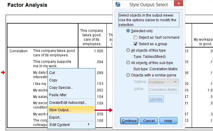
You can now make a selection of output items you'd like to modify. Personally, I think there's too many options here and it's unclear to me what they mean. I find it much easier to make my selection in the syntax. Clicking opens the main dialog.
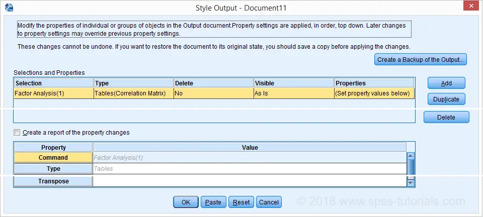
The main OUTPUT MODIFY dialog allows you to specify modifications for elements of your output items. I'll skip the details because -again- I find this easier to do this from syntax. In any case, the best syntax I could paste from the menu is shown below.
OUTPUT MODIFY Example - Pasted from Menu
OUTPUT MODIFY NAME=Document7
/REPORT PRINTREPORT=NO
/SELECT TABLES
/IF COMMANDS=["Factor Analysis(1)"] LABELS=[EXACT("Correlation Matrix")] INSTANCES=[1]
/DELETEOBJECT DELETE=NO
/OBJECTPROPERTIES VISIBLE=ASIS
/TABLECELLS SELECT=[CORRELATION] SELECTDIMENSION=COLUMNS SELECTCONDITION="Abs(x)>=0.5"
STYLE=REGULAR BOLD APPLYTO=CELL.
OUTPUT MODIFY - Syntax Problems
The syntax we just pasted is utter stupidity because it won't work in most situations; NAME=Document7 restricts the command to an output window named “Document7”. That's where my table resides now but probably not tomorrow when I continue working on my project. Let alone when a colleague or client tries to replicate my work. This defeats the whole point of working from syntax in the first place.
Furthermore, the syntax is way too long and complex to write manually but most of it does absolutely nothing. Now, most things in SPSS -including OUTPUT MODIFY- are best done by writing simple, clean syntax. Sadly, this pasted syntax is a very poor example for doing so. This goes for many other commands as well.
Last, "Abs(x) ≥ 0.5" includes the diagonal elements because abs(1.000) > 0.5. What I need is something like "Abs(x) ≥ 0.5 & Abs(x) < 1". I tried to accomplish this from the menu. I failed.
In short, I think
the pasted syntax sucks like hell
and I don't like the OUTPUT MODIFY dialogs either. So let's now study some examples that get things done the right way.
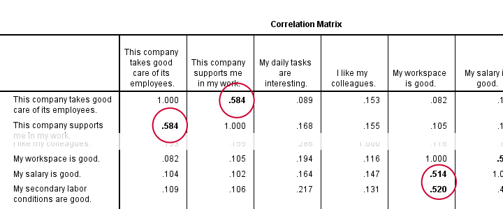
1. Boldface Correlations > 0.5
factor
/variables q1 to q9
/print correlation.
*Boldface absolute correlations > 0.5.
output modify
/select tables
/if commands = ['factor analysis'] subtypes = ['Correlation Matrix']
/tablecells select = [body] selectcondition = ["0.5 < abs(x) < 1"] style = bold.
Result
Notes
For processing all tables in the active output window, just use
OUTPUT MODIFY
/SELECT TABLES...
Optionally, specify some conditions by adding an /IF subcommand as in
OUTPUT MODIFY
/SELECT TABLES
/IF COMMANDS = ['FACTOR ANALYSIS']
Only tables that satisfy all conditions are processed. Confusingly, COMMANDS does not refer to the commands that created the output -FACTOR in this example.
Instead, COMMANDS refers to the OMS command identifiers which you can copy-paste from the output outline. The same goes for SUBTYPES and LABELS as shown below.
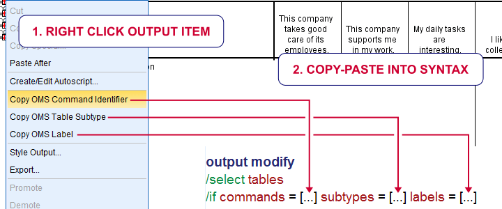
Now, the BODY of our table contains just correlations. If we set some condition, we refer to those as x as in
x > 0.5
So how to style absolute correlations between 0.50 and 1 (exclusive)? The obvious way seems
abs(x) > 0.5 & abs(x) < 1
but it somehow does not work. Instead,
0.5 < abs(x) < 1
does the job. However, it's a rather unusual way to formulate such a condition in SPSS.
Last but not least, OUTPUT MODIFY seems unable to undo the boldfacing exercise. Insofar as I understood, the syntax below should work but it doesn't.
output modify
/select tables
/if commands = ['factor analysis'] subtypes = ['Correlation Matrix']
/tablecells select = [body] selectcondition = ["0.5 < abs(x) < 1"] style = regular.
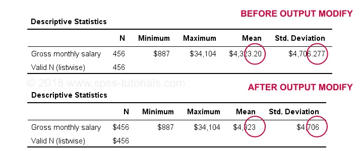
2. Set Decimal Places Output Tables - Example I
descriptives salary.
*Set format for all cells in last table -whatever that was- to dollar1 (zero decimal places).
output modify
/select tables
/if instances = [last] /*SELECT LAST PIVOT TABLE IN OUTPUT*/
/tablecells select = [body] format = 'dollar1'.
Result
Set Decimal Places Output Tables - Example II
descriptives q1 to q4.
descriptives q5 to q9.
*Set 2 decimal places for columns 4 and 5 for all descriptives tables in output.
output modify
/select tables
/if commands = ['descriptives'] /*SELECT ALL TABLES IN OUTPUT CREATED BY DESCRIPTIVES COMMAND*/
/tablecells select = [position(4) position(5)] selectdimension = columns format = 'f3.2'.
*Note: "[position(4) position(5)] selectdimension = columns" selects columns 4 and 5.
3. Transpose One or Many Output Tables
*Run 2 basic means tables.
means q1 to q4.
means q5 to q9.
*Transpose only last means table but not case processing summary.
output modify
/select tables
/if commands = ['means(last)'] subtypes = ['report'] /* SELECT ONLY "REPORT" (DESCRIPTIVES) TABLE CREATED BY LAST MEANS COMMAND */
/table transpose = yes.
Result
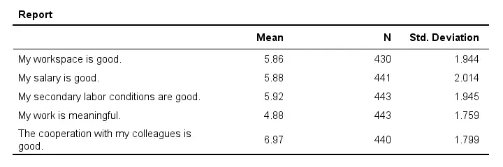
Notes
This example shows how to create much nicer descriptive statistics tables than using DESCRIPTIVES. Using MEANS instead results in a better table format and allows reporting the median as well as skewness and kurtosis without their standard errors. For more on this, see SPSS DESCRIPTIVES - Problems and Fixes.
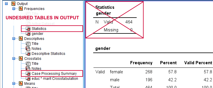
4. Delete Selection of Output Items
frequencies gender.
descriptives salary.
crosstabs educ by marit.
means salary by gender.
correlations salary with whours.
*Delete all unwanted tables: "statistics" for frequencies and "case processing summary" for means and descriptives.
output modify
/select tables
/if subtypes = ['case processing summary','statistics']
/deleteobject delete = yes.
Result
Notes
This example comes in very handy if you need to do some “quick and dirty” reporting to a client who doesn't have SPSS installed. In this case, delete all undesired output and convert the entire output document to PDF. You can do so by creating an OUTPUT EXPORT command from
![]() (only available in the output window).
(only available in the output window).
Alternativey, clean up your output window and convert everything in one go to an .rtf (rich text format, “WORD”) file. Since this'll include all tables and charts, you can use this as a great starting point for your final report.
5. Set Font Size for Output Tables
Note: this works properly for FREQUENCIES, DESCRIPTIVES and CORRELATIONS and only partly for MEANS and CROSSTABS.
frequencies gender.
descriptives salary.
crosstabs educ by marit.
means salary by gender.
correlations salary with whours.
*Set font sizes to 25 points.
output modify
/select tables
/tablecells select = [body,headers,title] fontsize = 25.
Result
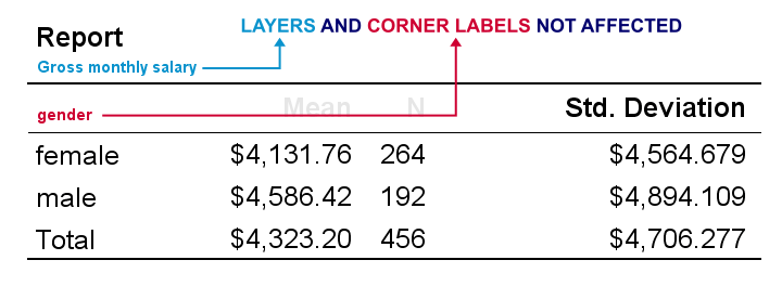
As we see, OUTPUT MODIFY seems unable to modify corner labels and layer dimensions. A workaround is creating a tablelook that sets a font size for all table elements. Next, OUTPUT MODIFY can apply this template to one, many or all output tables as shown below.
output modify
/select tables
/table tlook = "C:\Program Files\IBM\SPSS\Statistics\25\Looks\Original-15pt.stt".
*Shorthand if table template resides in default "Looks" folder (such as "C:\Program Files\IBM\SPSS\Statistics\25\Looks\").
output modify
/select tables
/table tlook = "Original-15pt".
*Don't use table template for any tables in output window.
output modify
/select tables
/table tlook = none.
Keep in mind that CD ignores the TLOOK setting, which is very annoying if your clients must replicate things on their own computers. You'll need to use absolute paths here and adjust those each time you move your project folder.
Alternatively, you can use a shorthand if you put your table templates in the default looks folder (such as C:\Program Files\IBM\SPSS\Statistics\24\Looks). However, that's typically where you don't want to develop, store and backup any project files.
6. Set Exact Size for Charts
frequencies dob
/format notable
/histogram.
*Set chart size to 720 by 300 points (resulted in 964 by 404 points).
output modify
/select charts
/objectproperties size=points(720,300).
Result
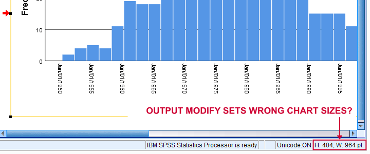
Apparently, OUTPUT MODIFY sets a different chart size than specified. For setting the correct chart sizes, try our SPSS - Set Chart Sizes Tool.
Final Notes
In this tutorial, I tried to cover the most important OUTPUT MODIFY tricks. But I still wonder:
“did I miss anything?”
If you -the reader- have any additional example(s) I should add to this tutorial, please drop me a comment below. Last but not least:
thanks for reading!
SPSS LAG Function – What and Why?
In SPSS, LAG is a function that returns the value of a previous case. It's mostly used on data with multiple rows of data per respondent. Here it comes in handy for calculating cumulative sums or counts.
 SPSS Lag Function
SPSS LAG - Basic Example 1
The most basic way to use LAG is COMPUTE V1 = LAG(V2). This simply computes a (possibly new) variable V1 holding the value of the previous case on V2. This is illustrated by the first screenshot. It's the result of running the syntax below. Since the first case doesn't have a previous case, it has a system missing value on the new variable.
SPSS LAG Syntax Example 1
data list free / id.
begin data
1 2 2 3 3 3 4 4 4 4
end data.
*2. Find id value of previous case.
compute previous_id = lag(id).
exe.
SPSS Lag - Creating a Counter
A great way to illustrate how LAG works is to create a counter variable. For each id value we'll create a variable that indicates its nth row of data. We'll start by identifying the first record of each id by using an IF command as shown in the syntax below. How it works is illustrated by the screenshot.
if $casenum = 1 or id ne lag(id) counter = 1.
exe.
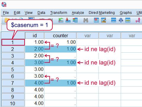 Identify first row for each id value
Next we'll finish our counter. What's important to understand here is that cases are processed sequentially from top to bottom when SPSS executes data transformations. That is, SPSS will start at $casenum = 1 and work its way down case by case. So a value created by LAG during this process may be used by the next case. The screenshot below illustrates three of the steps that occur while SPSS processes the syntax below.Since these steps usually require milliseconds to complete you don't actually see them occurring in normal situations.
if sysmis(counter) counter = lag(counter) + 1.
exe.
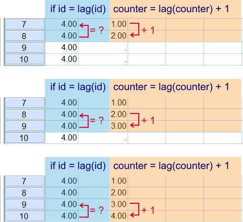 SPSS processes cases sequentially from top to bottom
SPSS Long Data Format
 SPSS Long Data Format. Note how each customer can have one or more records.
We'll continue with real world examples that gradually increase in level. Say we have data holding orders as records as in the figure above. Note that each customer can have one or several rows of data. This format is often referred to as a long data format.The opposite of this, with each customer's data on a single row, is called a wide data format. Relevant questions regarding these data may be
- How often do customers place an order? Or alternatively, how many days pass between orders by one customer?
- How many orders does the average customer place?
- How much money do customers spend?
We'll walk through these questions using the LAG function for answering them.
SPSS LAG Example - Days Between Orders
Running the syntax below will create the data from the previous screenshot and find the days between orders by one customer. Note that the records must first be sorted in a meaningful way. Next, if customer_id = lag(customer_id) checks whether each record is not the first record for a given customer. Only for these records days_between_orders will be calculated.
SPSS LAG Syntax Example 2
data list free / order_id (f2.0) order_date(edate10) customer_id invoice_amount (2f3.0).
begin data
1 26.09.2011 8 100 2 30.10.2011 8 100 3 28.12.2011 3 100 4 21.01.2012 12 150 5 26.01.2012 3 110
6 31.01.2012 7 140 7 16.02.2012 12 190 8 22.02.2012 12 30 9 23.02.2012 3 150 10 04.04.2012 12 50
end data.
*2. Sort records by customer_id and then order_date.
sort cases customer_id order_date.
*3. Compute days between orders by single customer.
if customer_id = lag(customer_id) days_between_orders = datediff(order_date,lag(order_date),'days').
exe.
SPSS LAG Example - Cumulative Orders per Customer
Now we'll create a cumulative order count per customer. We'll first set this new variable to 1 for each customer's first record. This is selected by if $casenum = 1 or lag(customer_id) ne customer_id. Next, we'll add 1 to it for each consecutive record if it belongs to the same customer. This condition is implied by if customer_id = lag(customer_id) Note that we make use of the fact that SUM(SYSTEM MISSING,X) = X. We can't use the + operator here because SYSTEM MISSING + X = SYSTEM MISSING.
SPSS LAG Syntax Example 3
if $casenum = 1 or lag(customer_id) ne customer_id cumulative_orders = 1.
exe.
*2. For each consecutive record, add 1 to cumulative_orders.
if customer_id = lag(customer_id) cumulative_orders = sum(lag(cumulative_orders),1).
exe.
SPSS LAG Example - Cumulative Expenditure
Finally we'll create the cumulative expenditure. This works quite similarly to the previous example. Instead of adding 1 to each consecutive record, we now add invoice_amount.
SPSS LAG Syntax Example 4
if $casenum = 1 or lag(customer_id) ne customer_id cumulative_amount = invoice_amount.
exe.
*2. Cumulative amount for second through nth records.
if customer_id = lag(customer_id) cumulative_amount = sum(invoice_amount,lag(cumulative_amount)).
exe.
 Original variables and those created by using LAG
Notes
- As a rule of thumb, always run
EXECUTEimmediately after commands usingLAG. This is one of the very few cases where you really need to runEXECUTEor a procedure.The reason for this is rather technical but for those who wonder:LAGis always carried out after all other transformations. This means that the order in which commands are executed may deviate from the order in which they're specified. So if a variable affected byLAGis used in a subsequent command, the latter is likely to use the ‘wrong’ values becauseLAGhasn't taken place yet. - In order to get the value of the nth previous case, use
LAG(...,n). Note thatnmust be a positive integer. That is, you can't useLAG(v1,-1)for getting the value from the next instead of the previous case.
Getting Values from Next Cases
LAGcan't readily access values from next rather than previous cases. If you do need the value of a next case, one option is to reverse the order of the cases and useLAGanyway.- You can also get values from next cases with
CREATEorSHIFT VALUES. Note that these are procedures (and not functions). This means you can't use them in anIFcommand for evaluating conditions like we did in most of the examples discussed in this tutorial.
Additional Examples
Shortly after writing this tutorial we received some more challenging questions that are solved by using mainly LAG and IF statements. We'll walk through them below.
SPSS Lag - Identifying Sessions
“We held an experiment in which respondents were presented with random pictures. Each picture may or may not occur repeatedly. Subsequent presentations of a single picture constitute a session. How can we add these sessions to our data?”
The syntax below focuses on explaining how things work, step by step. It's not the fastest option for answering the question.For one way to shorten it, see Compute A = B = C.
SPSS LAG Syntax Example 5
data list free / sequence id picture.
begin data.
1 1 1 2 1 4 3 1 3 4 1 4 5 1 4 6 1 4 7 1 1 8 1 1 9 1 3 10 1 3 1 2 3 2 2 3 3 2 3 4 2 4 5 2 2 6 2 4 7 2
1 8 2 2 9 2 3 10 2 1 1 3 1 2 3 3 3 3 3 4 3 4 5 3 4 6 3 2 7 3 1 8 3 4 9 3 3 10 3 3
end data.
variable labels id 'Respondent id'.
*.2 Session = 1 for every respondent's first row of data.
if $casenum eq 1 or id ne lag(id) session = 1.
exe.
*3. Detect switches (different picture for same respondent).
if $casenum gt 1 and id eq lag(id) and picture ne lag(picture) switch = 1.
exe.
*4. Increase session with 1 for every switch.
if $casenum ne 1 and id eq lag(id) session = sum(lag(session),switch).
exe.
*5. Optionally, delete "switch".
delete variables switch.
SPSS Lag - Count Votes in Households
“We collected data on different people in households. One of our variables, vote is the political party each respondent would vote for when asked. We'd like to estimate the political heterogeneity of households by counting the number of different values on vote. How can we do this?”
Note the use of AGGREGATE in step 6. As with the previous example, this syntax could be shortened.
SPSS LAG Syntax Example 6
data list free / household_member household vote.
begin data
1 1 4 1 2 3 2 2 3 3 2 1 4 2 1 5 2 4 1 3 3 2 3 4 1 4 1 2 4 4 1 5 2 2 5 2 3 5 3 4 5 4 5 5 1
end data.
*2. Sort by household, then vote.
sort cases by household vote.
*3. For first member of household, counter = 1.
if $casenum = 1 or household ne lag(household) counter = 1.
exe.
*4. Identify switches (vote changes within household).
if $casenum ne 1 and household = lag(household) and vote ne lag(vote) switch = 1.
exe.
*5. Increase counter by 1 for every switch.
if $casenum ne 1 and household = lag(household) counter = sum(lag(counter),switch).
exe.
*6. Different votes in household = max(counter).
aggregate outfile = * mode addvariables
/break household
/different_votes_in_household = max(counter).
*7. Optionally delete temp helper variables.
delete variables counter switch.
SPSS VARSTOCASES – What and Why?
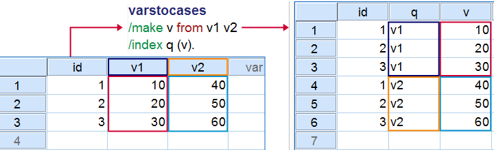
SPSS VARSTOCASES is short for “variables to cases”. It restructures data by stacking variables on top of each other as illustrated by the figure above. You can try this simple example for yourself by downloading and opening sav_data018 and running the syntax below on it.
SPSS VARSTOCASES Example 1
varstocases
/make v from v1 v2
/index q (v).
SPSS VARSTOCASES - Why?
One good reason for using VARSTOCASES is that many SPSS graphs can only be generated after stacking the relevant variables on top of each other. On top of that, VARSTOCASES also facilitates generating some tables. For example, let's take a look at some of the data in freelancers.sav.
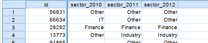
We may want to compare the sectors our respondents have been working in over years as in the table below.
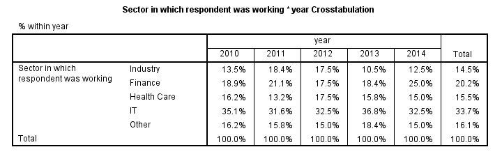
Makes sense, right? Now, one way for creating this table is CTABLES (custom tables) but this requires a (paid) add-on module. Second, TABLES will do the trick but it's available only in (challenging) syntax and no longer documented.
The third option is VARSTOCASES followed by CROSSTABS as demonstrated below. Note that VARSTOCASES results in an incorrect variable label so we correct that in step 2. We'll discuss this problem a bit later on.
SPSS VARSTOCASES Example 2
varstocases
/make sector from sector_2010 to sector_2014
/index year(sector).
*2. Correct variable label.
variable labels sector "Sector in which respondent was working".
*3. Extract year from string.
compute year = char.substr(year,index(year,'_') + 1).
execute.
*4. Generate table.
crosstabs sector by year/cells column.
SPSS VARSTOCASES - Creating Multiple Variables
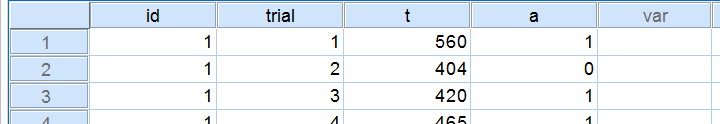
Our first two examples created one variable holding the original values and a second (index) variable holding the original variable names. In some cases, however, you may want to restructure multiple sets of variables in one go. For instance, let's consider sav_data016, holding typical reaction time data.
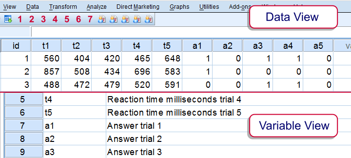
Apparently, respondents took 5 trials, each resulting in an answer and a reaction time. So do wrong answers have shorter or longer average reaction times? One way to figure out is using the VARSTOCASES syntax below, perhaps followed by MEANS.
SPSS VARSTOCASES Example 3
varstocases
/make t from t1 to t5
/make a from a1 to a5
/index trial.
Result
SPSS VARSTOCASES - Wrong Results
In our second example, we placed two variables on top of each other in one new variable. Both input variables had a variable label but the (single) output variable can have only one variable label. SPSS “solves” the problem by using the first variable label it encounters. In most cases, this will be incorrect but we'll readily see the problem.
The real problem with VARSTOCASES is that the same principle holds for value labels. This may result in nonsensical results. We'll now demonstrate this on sav_data017, part of which are shown below.
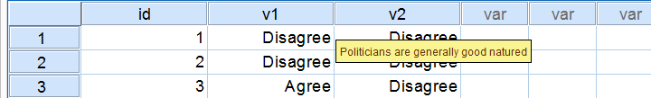
We first run basic FREQUENCIES. Note that both questions basically indicate that politicians are not very popular with our respondents.
set tnumbers both.
*2. Frequency tables.
frequencies v1 v2.
Result
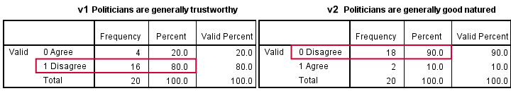
Importantly, these tables also show that our two variables have inconsistent value labels. We now run VARSTOCASES and replicate both frequency tables with a single contingency table.
SPSS VARSTOCASES Example 4
varstocases
/make v from v1 v2
/index question(v).
*2. Remove incorrect variable label.
variable labels v ''.
*3. Note that result is not correct.
crosstabs v by question/cells columns.
Result
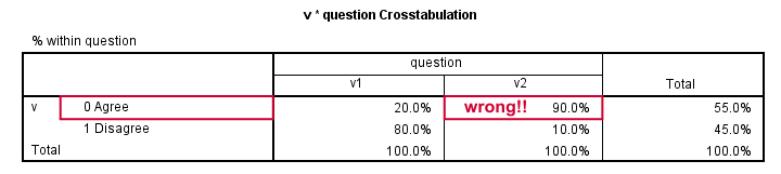
Note that VARSTOCASES has applied the value labels of v1 to the values of v1 and v2, resulting in misleading results. Even more disturbing, SPSS didn't throw any error or warning that things were going wrong at some point.
Believe it or not but this is not a bug. VARSTOCASES is supposed to work like this and this behavior is described in the CSR. We wonder, however, how many SPSS users are aware that this may happen. And even those who are aware have no efficient way for circumventing it as SPSS completely lacks any dictionary consistency check.
On a personal note, we feel that VARSTOCASES should perform such a check by default and at least issue a warning if things do go wrong. This suggestion goes for ADD FILES too, which shows similar problematic behavior which is even harder to avoid.
SPSS TEMPORARY Command
Summary
In SPSS, TEMPORARY indicates that the commands that follow are temporary. Temporary commands will be undone (reversed) when a command is run that reads the data. Such a command also indicates that the commands that follow are not temporary anymore.
 Temporary commands between TEMPORARY and a command that reads the data.
SPSS Temporary Example
“We'd like to dichotomize customer satisfaction into "satisfied" and "not satisfied". Next, we'd like to see its relation to perceived quality. For each category of the latter, we want to see the percentage of satisfied customers.”
We'll first create and label our dichotomous variable. Next, we'll modify its format a bit but only for the requested table. By using TEMPORARY we don't need to undo these modifications after creating the table. The syntax below demonstrates this. It uses supermarket.sav.
SPSS Temporary Syntax Example
compute satisfied = v1 ge 4.
*2. Apply clear labels to our new variable.
variable labels satisfied "Dichotomized version of v1".
value labels satisfied 0 "Not satisfied" 1 "Satisfied".
*3. Start temporary commands.
temporary.
*4. Temporary commands for showing percentages in table.
compute satisfied = 100 * satisfied.
formats satisfied(pct3.0).
variable labels satisfied "Percentage of satisfied customers".
*5. Creating table reads data and reverses temporary commands.
means satisfied by v5 /cells mean.
*6. Temporary commands have been undone now.
means satisfied by v5 /cells mean.
Note that the second MEANS command is identical to the first one. Its output is different because the temporary modifications that affect the first table have been undone by the first MEANS command.
 Same command, different results
Which Commands Read the Data?
In order to use TEMPORARY effectively, you must know which commands do or do not read the data.What reading the data means in the first place is discussed in SPSS Procedures.An easy option for finding this out is consulting the command syntax reference. Where relevant, it explicitly states whether a command reads the data. When in doubt, experienced users can probably just reason out whether a command reads the data or not.
Which Commands are Affected by Temporary?
As a rule of thumb
- all of the transformations and dictionary modifications but
- none of the procedures
can be used with TEMPORARY. For a complete and more accurate overview, consult the CSR.
SPSS TableLooks – Quick Introduction
SPSS TableLooks are files that contain styling
-colors, fonts, borders and more- for SPSS output tables.
- What can I (not) do with TableLooks?
- Applying TableLooks
- Creating TableLooks
- Developing TableLooks
- Issues with TableLooks
 Output Table Styled by TableLook Example
Practice Data File
This tutorial uses bank_clean.sav throughout. Part of its data view is shown below. Feel free to download these data and try the examples we'll run for yourself.
What are TableLooks?
SPSS TableLooks are tiny text files written in XML. They contain styling for output tables such as
- colors for text, backgrounds and borders;
- fonts: sizes, families and styles;
- widths for columns and row labels but -unfortunately- not entire tables;
- which borders to apply in which widths and colors.
TableLooks have the .stt file extension (.stt is short for SPSS table template, the old name for TableLooks). SPSS ships with some TableLooks which you find in the Looks subfolder as shown below.
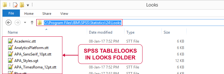
Ironically, some of these TableLooks don't work because they contain errors. But we'll get to that later.
Some things TableLooks can't do are
- applying conditional styling such as boldfacing correlations that are statistically significant;
- setting numeric formats for SPSS output such as decimal places and percent signs.
For these modifications, try OUTPUT MODIFY instead.
Applying TableLooks
Let's first create a very simple means table. The fastest way to do so is running the following line of syntax: means salary by jtype. If you're on SPSS version 23 or higher, the resulting table looks awful.
 Default Table Styling for SPSS 23 and Higher
However, if we set a different TableLook and rerun the table, it'll look way better. The syntax below does just that. Note that you probably need to change the path to your Looks folder.
Set TableLook and Rerun Means Table
set tlook 'C:\Program Files\IBM\SPSS\Statistics\24\Looks\APA_TimesRoma_12pt.stt'.
*Rerun basic means table.
means salary by jtype.
Result
This already looks much better, doesn't it? However, the text alignment is somewhat awkward and does not follow APA guidelines. Can't we do better? Yes we can.
Creating TableLooks
Let's double-click this last table and open the menu as shown below. If it looks different, make sure you double-click the table. We'll briefly discuss its main options below.
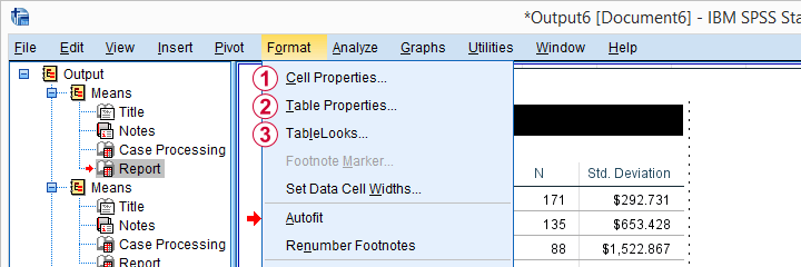
Set properties for a selection of table cells here. However, these changes can't be saved as a TableLook (.stt) file.
Set properties for table areas -titles, headers, data cells- here. These changes can be saved as a TableLook.
After editing some table, save its styling as a TableLook here.
Since we'd like to make changes that we can save as a TableLook, we choose Table Properties. We can now set styles for different table areas as shown below.
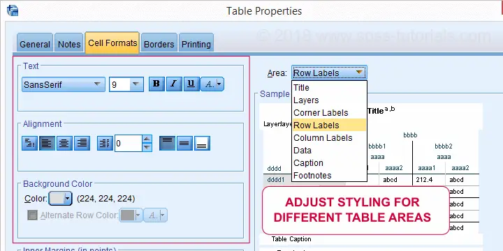
When we're done, we'll double-click our table again and select TableLooks. We can now save the styling we just applied as a new or existing TableLook (.stt) file.
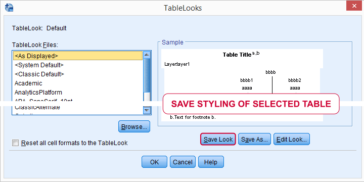
We can now activate our TableLook by running something like set tlook 'd:/data/myNewTableLook.stt'. From now on, all tables we'll create will look great! Like the one shown below, for example.
Output Table Styled by TableLook Example
If you want to revert to the ugly SPSS defaults, you can do so by running set tlook none.
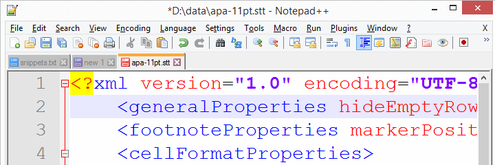
Developing TableLooks
If you're not afraid of code, there's a faster way to develop TableLooks: you can edit their XML directly in some text editor such as Notepad++. The screenshot below shows what that looks like.
Issues with TableLooks
As we already mentioned, some TableLooks developed by IBM SPSS don't work in recent SPSS versions. For an example, try and run the syntax below.
set tlook 'C:\Program Files\IBM\SPSS\Statistics\25\Looks\LargeFont.stt'.
*Running table triggers warning and ugly default styling is used.
frequencies jtype.
Result
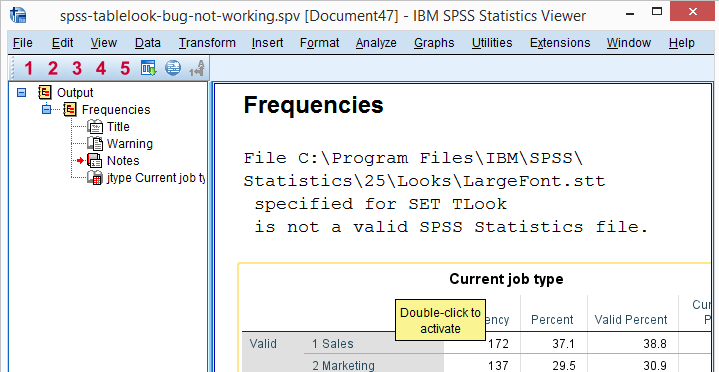
So when we activate this TableLook, everything seems fine. However, as soon as we actually run some table, we get the following warning: File C:\Program Files\IBM\SPSS\Statistics\25\Looks\LargeFont.stt specified for SET TLook is not a valid SPSS Statistics file. This warning comes up whenever a TableLook file contains errors. Which is somewhat ironic for a TableLook that ships with SPSS.
A second issue with SET TLOOK is that it ignores the CD setting. I always deliver entire projects -all data, syntax, output and templates- to my clients. This allows them to replicate exactly everything I did. I really feel that
this should be the standard for any professional.
Right, so my clients usually download the project folder holding all necessary files. Next, they only need to change the CD setting and
- GET opens the right data file,
- SET CTEMPLATE sets the right chart templates,
- INSERT runs the right syntax files and
- OUPUT SAVE saves the output in the right folder and then
- SET TLOOK crashes
for no apparent reason. It would be nice if this annoying issue would be fixed rather than just mentioned in the documentation.
Right, I guess that'll do for a quick introduction to SPSS TableLooks. Hope you found it helpful.
Thanks for reading!
SPSS EXECUTE – What and Why?
EXECUTE runs pending transformations.
However, many SPSS users don't have a clue what that means. More importantly, when should you (not) run EXECUTE? And when do you really need it?
Let's dive in. We'll use adratings.sav throughout, part of which is shown below.
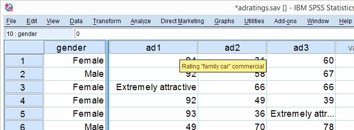
SPSS “Transformations Pending”
As you probably figured out, our data hold 18 respondents who rated 3 different advertisements. Now let's say we need to compute a corrected version of ad1 which we'll name cad1 by adding 10 points to each score.
The easy way is a simple COMPUTE command like
compute cad1 = ad1 + 10.
If you run just this syntax, your data view will look like below.
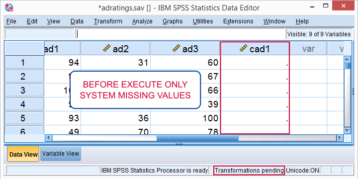
So what's “transformations pending” in the status bar? And where's my corrected scores? I told SPSS to compute them and it hasn't done so! F!@#$%g SPSS!
However, just running
execute.
successfully completes our transformation.
So Why Did we Need EXECUTE?
Basically everything we do in SPSS is done by commands. You may not see those if you work directly from the menu -a recipe for disaster as explained in SPSS Syntax - Six Reasons you Should Use it.
But anyway, SPSS commands come in 3 basic types:
- procedures are commands that must inspect all cases. Some examples are FREQUENCIES, DESCRIPTIVES and SORT CASES plus all charts and statistical tests. These commands require SPSS to “go through” all cases straight away.
- transformations are commands that will inspect all cases but this only happens when really needed. Well known transformations are COMPUTE, RECODE, IF and SELECT IF.
- other commands that don't inspect any cases. Examples are FILTER, VARIABLE LABELS and ADD VALUE LABELS.
If you want to know if a command is a procedure, transformation or other, consult Overview All SPSS Commands.Yes, I know. I need to update it. Any volunteer for that?
Now imagine that you're SPSS -it isn't hard to do. You have data with 100,000 cases open. If somebody asks you to COMPUTE something, you must go through all 100,000 cases. Quite a job!
Then, if the user asks for FREQUENCIES, you must go through all 100,000 cases again. So in order to save computing time (and electricity)
SPSS prefers to go through all cases just once
and do the COMPUTE and FREQUENCIES in one go. So that's why it won't immediately execute some commands -which are known as transformation commands.
SPSS Transformation Commands
Now if we consult the command syntax reference on COMPUTE, we see the following:
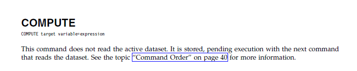 COMPUTE is a Transformation
The phrase “it is stored, pending” indicates that COMPUTE is a transformation. This means that we need to EXECUTE it if we want to inspect the result in the data editor before proceeding.
SPSS Procedures
If we look up FREQUENCIES, the fine manual tells us that
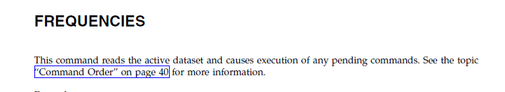 FREQUENCIES is a Procedure
and a command that “reads the active dataset” is a procedure.
This means that
running EXECUTE right before FREQUENCIES is pointless
and merely slows down SPSS.
The same goes for EXECUTE right after VARIABLE LABELS or RENAME VARIABLES: these are not transformations but take place immediately so there aren't any pending transformations to execute.
Importantly, some commands that transform your data are technically procedures, not transformations. Examples are ALTER TYPE, AGGREGATE and RANK.
So When To Use EXECUTE?
- Use EXECUTE if you have transformations pending and you want to visually inspect results before doing anything else.
- In rare cases, you need EXECUTE in order for your syntax to run correctly.
So when do you really need EXECUTE? I'm familiar with 3 scenarios so I'll present them below. Again, all examples use adratings.sav.
1. EXECUTE Before DELETE VARIABLES
compute total = sum(ad1 to ad3).
delete variables ad1 to ad3.
*Right way to compute total and delete input variables.
compute total = sum(ad1 to ad3).
execute.
delete variables ad1 to ad3.
2. EXECUTE Before LAG Function
compute prev_ad1 = lag(ad1).
compute ad1 = ad1 + 10.
execute.
*Right way to compute ad1 for previous case, then add 10 to original ad1.
compute prev_ad1 = lag(ad1).
execute.
compute ad1 = ad1 + 10.
execute.
3. EXECUTE After Using $Casenum
compute casenum = $casenum.
select if casenum > 10.
execute.
*Right way to delete first 10 cases.
compute casenum = $casenum.
execute.
select if casenum > 10.
execute.
I guess that's about it. Hope you liked it. Do you have any other examples in which you really need EXECUTE? Please drop me a comment below and let me know.
Thanks for reading!