SPSS Z-Test for a Single Proportion

• Z-Test - Assumptions
• SPSS Z-Test Dialogs
• SPSS Z-Test Output
• APA Style Reporting Z-Tests
• References

A z-test for a single proportion tests
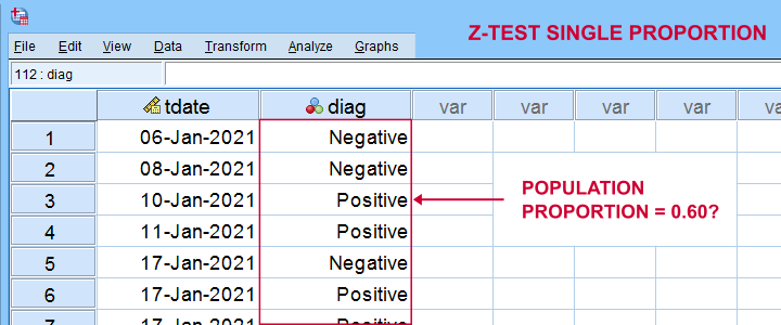
if some population proportion is equal to x. Example: does a proportion of 0.60 (or 60%) of all Dutch citizens test positive on Covid-19?

In order to find out, a scientist tested a simple random sample of N = 112 people. The results thus gathered are in covid-z-test.sav, partly shown below.

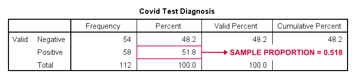
The first thing we'd like to know is: what's our sample proportion anyway? We'll quickly find out by running a single line of SPSS syntax: frequencies diag. The resulting table tells us that 51.8% (a proportion of .518) of our sample tested positive on Covid-19.

Now, does our sample outcome of 51.8% really contradict our null hypothesis that 60% of our entire population is infected? A z-test for a single proportion answers just that. However, it does require a couple of assumptions.

Z-Test - Assumptions

A z-test for a single proportion requires two assumptions:

• independent observations;
• \(n_1 \ge 15\) and \(n_2 \ge 15\): our sample should contain at least some 15 observations for either possible outcome.

Standard textbooks^3,5 often propose \(n_1 \ge 5\) and \(n_2 \ge 5\) but recent studies suggest that these sample sizes are insufficient for accurate test results.² For small sample sizes, the Agresti-Coull adjustment may somewhat improve your results.

A quick check for the sample sizes assumption is inspecting basic frequency distributions for the outcome variables. We already did this for our example data. Our outcomes -Covid negative or positive- have frequencies of 54 and 58 observations.

SPSS Z-Test Dialogs

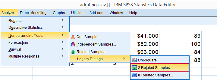
Starting from SPSS version 27, z-tests are found under Analyze Compare Means One-Sample Proportions For our example study, we'll fill in the dialogs as shown below.

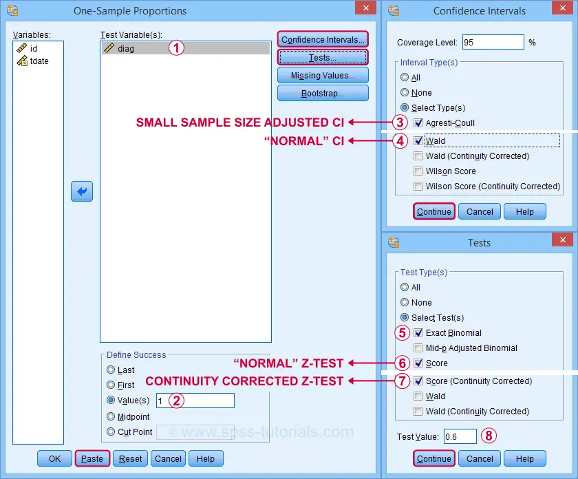
Our hypothesis addresses the proportion of positive tests, which is coded as 1 in our data.
Precisely, we hypothesized a population proportion of 0.60 (or 60%) to test positive for Covid-19.

Selecting these options results in the syntax below. Let's run it.

SPSS Z-Test Output

The first output table presents 95% confidence intervals for our population proportion.

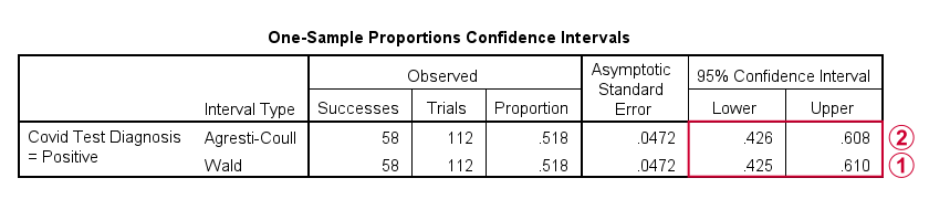
The “normal” confidence interval (denoted as Wald) runs from .425 to .610: there's a 95% probability that these bounds enclose our population proportion. Also note that our hypothesized proportion of .60 lies within this interval of likely values.

The Agresti-Coull interval is probably a worse estimate than our “normal” confidence interval unless the sample sizes assumption is not met. I recommend ignoring it for our example data.

The second table presents the actual z-test results.

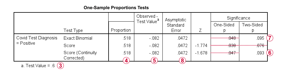
Our hypothesized population proportion is .60.
Our observed sample proportion is .518.
The observed difference is .518 - .60 = -.082.

The continuity corrected significance level is always more accurate than the uncorrected p-value. For our example, p(2-tailed) = .093. Because p > .05, we do not reject the null hypothesis that our population proportion = .60. That is, the difference of -.082 is not statistically significant.

The binomial test yields an exact 1-tailed p-value. Its 2-tailed p-value, however, is not correct: it's exactly 2 * p(1-tailed) but this calculation is only valid if the test proportion is 0.50.

For test proportions other than 0.50, the binomial distribution is asymmetrical. This is why the “traditional” binomial test in SPSS doesn't report any p(2-tailed) in this case as can be verified by the syntax below.

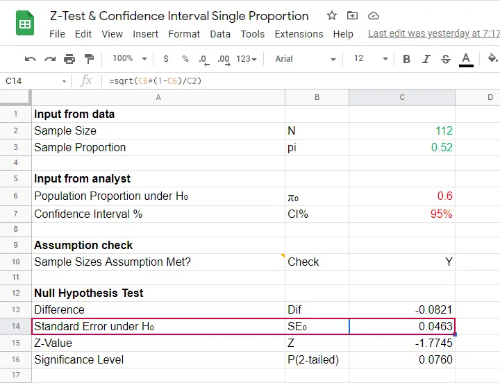
Finally, note that SPSS reports the wrong standard error. The correct standard error is .0463 as computed in this Googlesheet (read-only).

APA Style Reporting Z-Tests

The APA does not have explicit guidelines on reporting z-tests. However, it makes sense to report something like “the proportion of positive Covid-19 diagnoses did not differ significantly from 0.60, z = -1.68, p(2-tailed) = .093.” Obviously, you should also report

• your sample size;
• the observed sample proportion;
• whether the continuity correction was applied to the z-test;
• whether the Agresti-Coull correction was applied to the confidence interval.

Final Notes

Altogether, I think z-tests are rather poorly implemented in SPSS:

• the standard error for the z-test is not correct;
• p(2-tailed) for the binomial test is not correct;
• no warning is issued if sample sizes are even way insufficient to run a z-test in the first place;
• no effect size measures (such as Cohen’s H) are available;
• z-tests and confidence intervals are reported in separate tables which the end user will probably want to merge in Excel or something.

What's really good, however, is that

• z-tests in SPSS handle (even a combination of) numeric and string variables;
• several corrections for both the z-test and confidence intervals are available.

Thanks for reading!

References

1. Agresti, A. & Coull, B.A. (1998). Approximate Is Better than "Exact" for Interval Estimation of Binomial Proportions The American Statistician, 52(2), 119-126.
2. Agresti, A. & Franklin, C. (2014). Statistics. The Art & Science of Learning from Data. Essex: Pearson Education Limited.
3. Van den Brink, W.P. & Koele, P. (1998). Statistiek, deel 2 [Statistics, part 2]. Amsterdam: Boom.
4. Van den Brink, W.P. & Koele, P. (2002). Statistiek, deel 3 [Statistics, part 3]. Amsterdam: Boom.
5. Twisk, J.W.R. (2016). Inleiding in de Toegepaste Biostatistiek [Introduction to Applied Biostatistics]. Houten: Bohn Stafleu van Loghum.

SPSS Z-Test for Independent Proportions Tutorial

• Z-Test - Assumptions
• SPSS Z-Tests Dialogs
• SPSS Z-Test Output
• SPSS Z-Tests - Strengths & Weaknesses
• APA Reporting Z-Tests

A z-test for independent proportions tests if 2 subpopulations
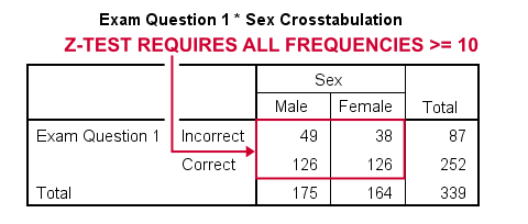
score similarly on a dichotomous variable. Example: are the proportions (or percentages) of correct answers equal between male and female students?

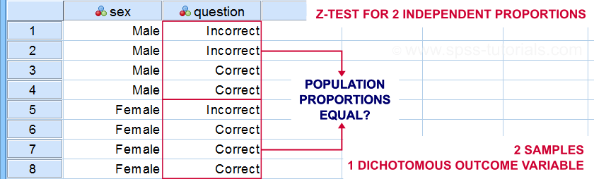
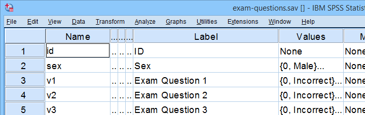
Although z-tests are widely used in the social sciences, they were only introduced in SPSS version 27. So let's see how to run them and interpret their output. We'll use exam-questions.sav -partly shown below- throughout this tutorial.

Now, before running the actual z-tests, we first need to make sure we meet their assumptions.

Z-Test - Assumptions

Z-tests for independent proportions require 2 assumptions:

• independent observations and
• sufficient sample sizes.

Regarding this second assumption, Agresti and Franklin (2014)² propose that both outcomes should occur at least 10 times in both samples. That is,

$$p_a n_a \ge 10, (1 - p_a) n_a \ge 10, p_b n_b \ge 10, (1 - p_b) n_b \ge 10$$

where

• \(n_a\) and \(n_b\) denote the sample sizes of groups a and b and
• \(p_a\) and \(p_b\) denote the proportions of “successes” in both groups.

Note that some other textbooks^3,4 suggest that smaller sample sizes may be sufficient. If you're not sure about meeting the sample sizes assumption, run a minimal CROSSTABS command as in crosstabs v1 to v5 by sex. As shown below, note that all 5 exam questions easily meet the sample sizes assumption.

For insufficient sample sizes, Agresti and Caffo (2000)¹ proposed a simple adjustment for computing confidence intervals: simply add one observation for each outcome to each group (4 observations in total) and proceed as usual with these adjusted sample sizes.

SPSS Z-Tests Dialogs

First off, let's navigate to Analyze Compare Means Independent-Samples Proportions and fill out the dialogs as shown below.

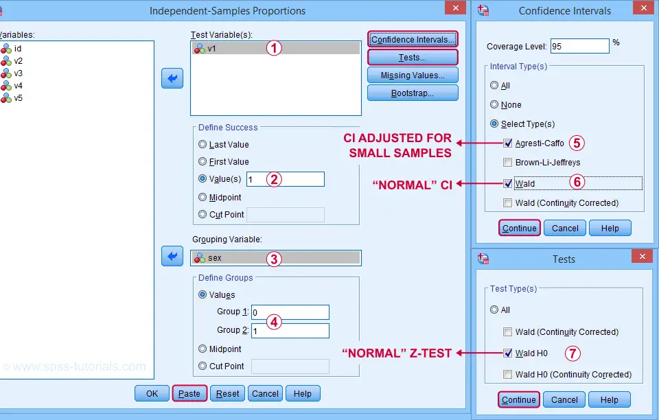
Clicking “Paste” results in the SPSS syntax below. Let's run it.

SPSS Z-Test Output

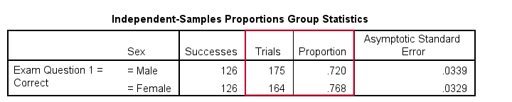
The first table shows the observed proportions for male and female students. Note that female students seem to perform somewhat better: a proportion of .768 (or 76.8%) answered correctly as compared to .720 for male students.

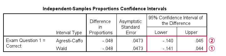
The second output table shows that the difference between our sample proportions is -.048.

The “normal” 95% confidence interval for this difference (denoted as Wald) is [-.141, .044]. Note that this CI encloses zero: male and female populations performing equally well is within the range of likely values.

I don't recommend reporting the Agresti-Caffo corrected CI unless your data don't meet the sample sizes assumption.

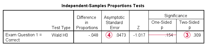
The third table shows the z-test results. First note that p(2-tailed) = .309. As a rule of thumb, we reject the null hypothesis if p < 0.05 which is not the case here. Conclusion: we do not reject the null hypothesis that the population difference is zero. That is: the sample difference of -.048 is not statistically significant.

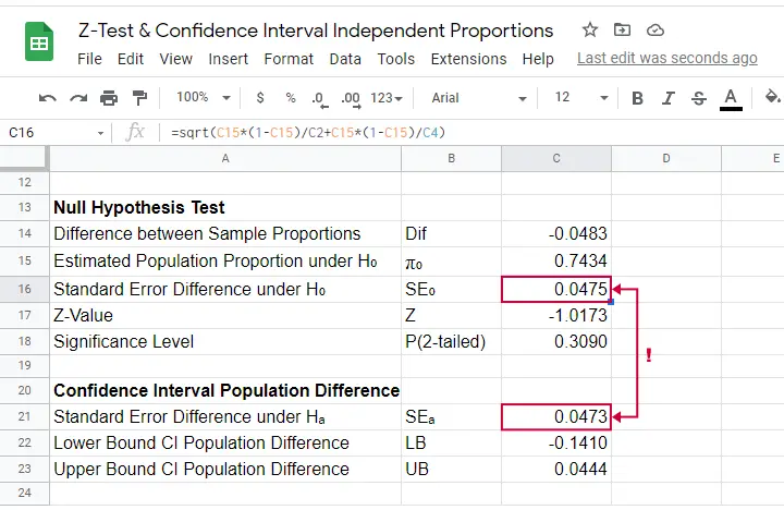
Finally, note that SPSS reports the wrong standard error for this test. The correct standard error is 0.0475 as computed in this Googlesheet (read-only) shown below.

SPSS Z-Tests - Strengths and Weaknesses

What's good about z-tests in SPSS is that

• you can analyze many dependent variables in one go;
• both the independent and dependent variables may be either string variables or numeric variables;We also tested SPSS z-tests on a mixture of string and numeric dependent variables. Although doing so is very awkward, the results were correct.
• many corrections -such as Agresti-Caffo- are available.

However, what I really don't like about SPSS z-tests is that

• no warning is issued if the sample sizes assumption isn't met;
• no effect size measures are available. Cohen’s H seems completely absent from SPSS and phi coefficients are available from CROSSTABS or CORRELATIONS;
• SPSS reports the wrong standard error for the actual z-test;
• z-tests and confidence intervals are reported in separate tables. I'd rather see these as different columns in a single table with one row per dependent variable.

APA Reporting Z-Tests

The APA guidelines don't explicitly mention how to report z-tests. However, it makes sense to report something like the difference between males and females
was not significant, z = -1.02, p(2-tailed) = .309. You should obviously report the actual proportions and sample sizes as well. If you analyzed multiple dependent variables, you may want to create a table showing

• both proportions being compared;
• the difference between the proportions and its confidence interval;
• z and p(2-tailed) for the null hypothesis of equal population proportions;
• some effect size measure.

References

1. Agresti, A & Caffo, B. (2000). Simple and Effective Confidence Intervals for Proportions and Differences of Proportions. The American Statistician, 54(4), 280-288.
2. Agresti, A. & Franklin, C. (2014). Statistics. The Art & Science of Learning from Data. Essex: Pearson Education Limited.
3. Twisk, J.W.R. (2016). Inleiding in de Toegepaste Biostatistiek [Introduction to Applied Biostatistics]. Houten: Bohn Stafleu van Loghum.
4. Van den Brink, W.P. & Koele, P. (2002). Statistiek, deel 3 [Statistics, part 3]. Amsterdam: Boom.

SPSS Sign Test for One Median – Simple Example

A sign test for one median is often used instead of a one sample t-test when the latter’s assumptions aren't met by the data. The most common scenario is analyzing a variable which doesn't seem normally distributed with few (say n < 30) observations. For larger sample sizes the central limit theorem ensures that the sampling distribution of the mean will be normally distributed regardless of how the data values themselves are distributed.
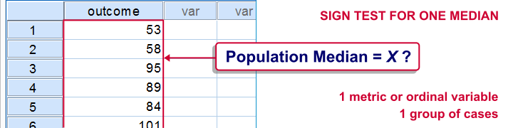
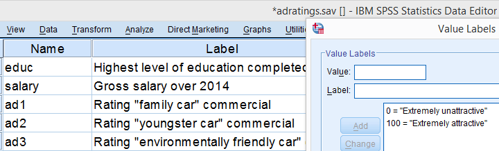
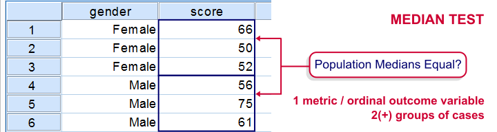
This tutorial shows how to run and interpret a sign test in SPSS. We'll use adratings.sav throughout, part of which is shown below.

SPSS Sign Test - Null Hypothesis

A car manufacturer had 3 commercials rated on attractiveness by 18 people. They used a percent scale running from 0 (extremely unattractive) through 100 (extremely attractive). A marketeer thinks a commercial is good if at least 50% of some target population rate it 80 or higher.
Now, the score that divides the 50% lowest from the 50% highest scores is known as the median. In other words, 50% of the population scoring 80 or higher is equivalent to our null hypothesis that the population median is at least 79.5 for each commercial. If this is true, then the medians in our sample will be somewhat different due to random sampling fluctuation. However, if we find very different medians in our sample, then our hypothesized 79.5 population median is not credible and we'll reject our null hypothesis.

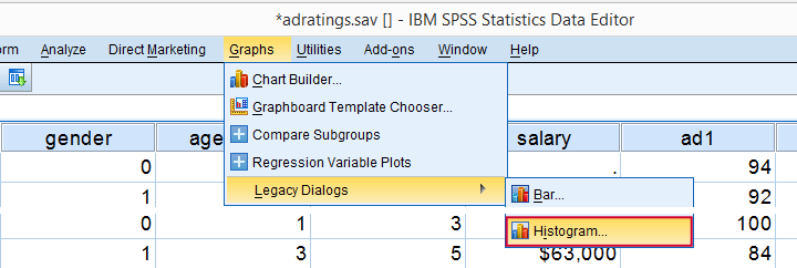
Quick Data Check - Histograms

Let's first take a quick look at what our data look like in the first place. We'll do so by inspecting histograms over our outcome variables by running the syntax below.

Result

First, note that all distributions look plausible. Since n = 18 for each variable, we don't have any missing values. The distributions don't look much like normal distributions. Combined with our small sample sizes, this violates the normality assumption required by t-tests so we probably shouldn't run those.

Quick Data Check - Medians

Our histograms included mean scores for our 3 outcome variables but what about their medians? Very oddly, we can't compute medians -which are descriptive statistics- with DESCRIPTIVES. We could use FREQUENCIES but we prefer the table format we get from MEANS as shown below.

SPSS - Compute Medians Syntax

Result

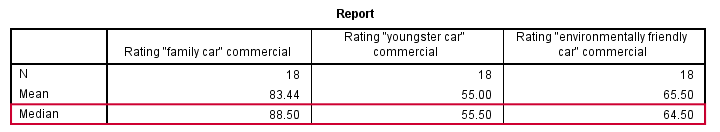
Only our first commercial (“family car”) has a median close to 79.5. The other 2 commercials have much lower median. But are they different enough for rejecting our null hypothesis? We'll find out in a minute.

SPSS Sign Test - Recoding Data Values

SPSS includes a sign test for two related medians but the sign test for one median is absent. But remember that our null hypothesis of a 79.5 population median is equivalent to 50% of the population scoring 80 or higher. And SPSS does include a test for a single proportion (a percentage divided by 100) known as the binomial test. We'll therefore just use binomial tests for evaluating if the proportion of respondents rating each commercial 80 or higher is equal to 0.50.
The easy way to go here is to RECODE our data values: values smaller than the hypothesized population median are recoded into a minus (-) sign. Values larger than this median get a plus (+) sign. It's these plus and minus signs that give the sign test its name. Values equal to the median are excluded from analysis so we'll specify them as missing values.

SPSS RECODE Syntax

SPSS Binomial Test Menu

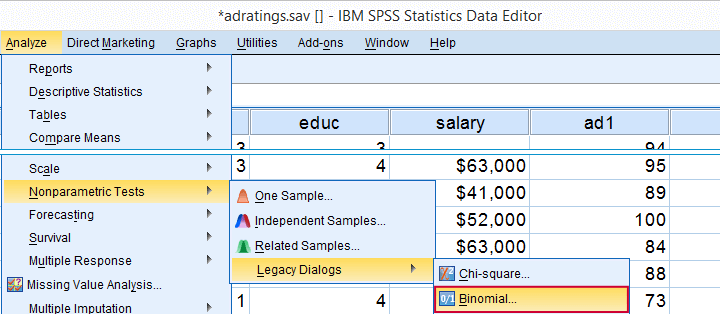
Minor note: the binomial test is a test for a single proportion, which is a population parameter. So it's clearly not a nonparametric test. Unfortunately, “nonparametric tests” often refers to both nonparametric and distribution free tests -even though these are completely different things.

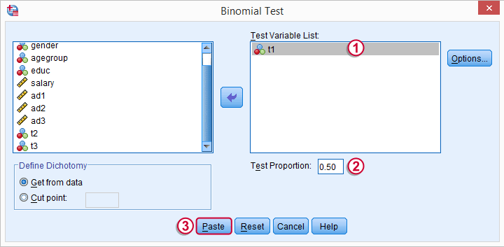
t1 is one of our newly created variables. It merely indicates if ad1 was 80 or higher. Completing the steps results in the syntax below.

SPSS Binomial Test Syntax

Modifying Our Syntax

Oddly, SPSS’ binomial test results depend on the (arbitrary) order of cases: the test proportion applies to the first value encountered in the data. This is no major issue if -and only if- our test proportion is 0.50 but it still results in messy output. We'll avoid this by sorting our cases on each test variable before each test.

Modified Binomial Test Syntax

Binomial Test Output

We'll first limit our focus to the first table of test results as shown below.

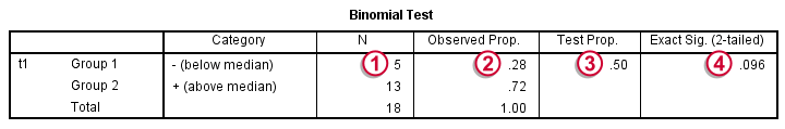
N: 5 out of 18 cases score higher than 79.5;
the observed proportion is (5 / 18 =) 0.28 or 28%;
the hypothesized test proportion is 0.50;
p (denoted as “Exact Significance (2-tailed)”) = 0.096: the probability of finding our sample result is roughly 10% if the population proportion really is 50%. We generally reject our null hypothesis if p < 0.05 so our binomial test does not refute the hypothesis that our population median is 79.5. Before we move on, let's take a close look at what our 2-tailed p-value of 0.096 really means.

The Binomial Distribution

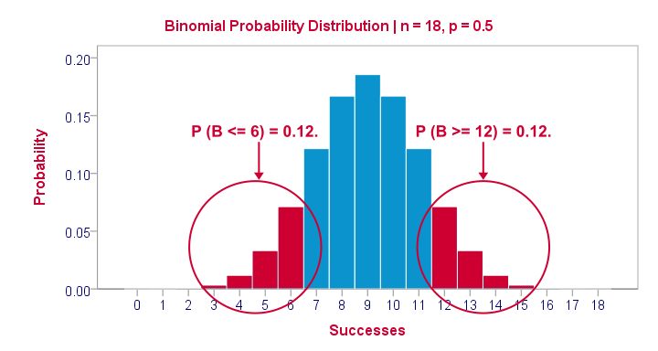
Statistically, drawing 18 respondents from a population in which 50% scores 80 or higher is similar to flipping a balanced coin 18 times in a row: we could flip anything between 0 and 18 heads. If we repeat our 18 coin flips over and over again, the sampling distribution of the number of heads will closely resemble the binomial distribution shown below.

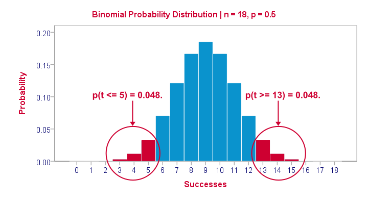
The most likely outcome is 9 heads with a probability around 0.19 or 19%. P = 0.048 for outcomes of 5 or fewer heads (red area). Now, reporting this 1-tailed p-value suggests that none of the other outcomes would refute the null hypothesis. This does not hold because 13 or more heads are also highly unlikely. So we should take into account our deviation of 4 heads from the expected 9 heads in both directions and add up their probabilities. This results in our 2-tailed p-value of 0.096.

Binomial Test - More Output

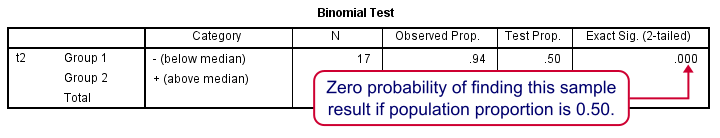
We saw previously that our second commercial (“youngster car”) has a sample median of 55.5. Our p-value of 0.000 means that we've a 0% probability of finding this sample median in a sample of n = 18 when the population median is 79.5. Since p < 0.05, we reject the null hypothesis: the population median is not 79.5 but -presumably- much lower. We'll leave it as an exercise to the reader to interpret the third and final test.

That's it for now. I hope this tutorial made clear how to run a sign test for one median in SPSS. Please let us know what you think in the comment section below. Thanks!

SPSS Sign Test for Two Medians – Simple Example

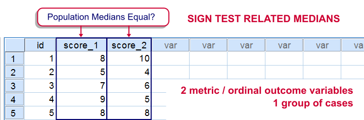
The sign test for two medians evaluates if 2 variables measured on 1 group of cases are likely to have equal population medians.There's also a sign test for comparing one median to a theoretical value. It's really very similar to the test we'll discuss here. Also see SPSS Sign Test for One Median - Simple Example . It can be used on either metric variables or ordinal variables. For comparing means rather than medians, the paired samples t-test and Wilcoxon signed-ranks test are better options.

Adratings Data

We'll use adratings.sav throughout this tutorial. It holds data on 18 respondents who rated 3 car commercials on attractiveness. Part of its dictionary is shown below.

Descriptive Statistics

Whenever you start working on data, always start with a quick data check and proceed only if your data look plausible. The adratings data look fine so we'll continue with some descriptive statistics. We'll use MEANS for inspecting the medians of our 3 rating variables by running the syntax below.DESCRIPTIVES may seem a more likely option here but -oddly- does not include medians - even though these are clearly “descriptive statistics”.

SPSS Syntax for Inspecting Medians

SPSS Medians Output

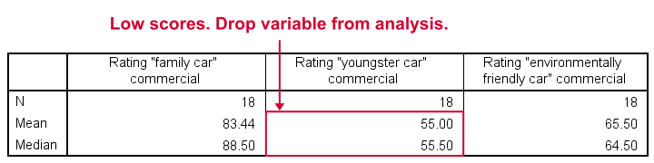
The mean and median ratings for the second commercial (“Youngster Car”) are very low. We'll therefore exclude this variable from further analysis and restrict our focus to the first and third commercials.

Sign Test - Null Hypothesis

For some reason, our marketing manager is only interested in comparing median ratings so our null hypothesis is that the two population medians are equal for our 2 rating variables. We'll examine this by creating a new variable holding signs:

• respondents who rated ad1 < ad3 receive a minus sign;
• respondents who rated ad1 > ad3 get a plus sign.

If our null hypothesis is true, then the plus and minus signs should be roughly distributed 50/50 in our sample. A very different distribution is unlikely under H0 and therefore argues that the population medians probably weren't equal after all.

Running the Sign Test in SPSS

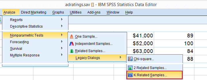
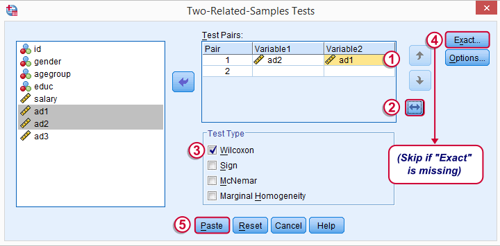
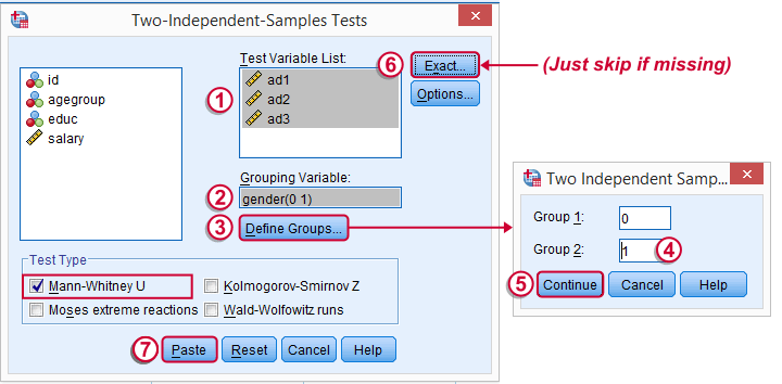
The most straightforward way for running the sign test is outlined by the screenshots below.

The 2 Related samples refer to the two rating variables we're testing. They're related (rather than independent) because they've been measured on the same respondents.

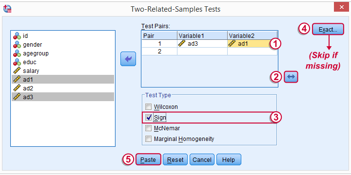
We prefer having the best rated variable in the second slot. We'll do so by reversing the variable order.
Whether your menu includes the Exact button depends on your SPSS license. If it's absent, just skip the step shown below.

SPSS Sign Test Syntax

Completing these steps results in the syntax below (you'll have one extra line if you included the exact test). Let's run it.

Output - Signs Table

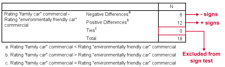
First off, ties (that is: respondents scoring equally on both variables) are excluded from this analysis altogether. This may be an issue with typical Likert scales. The percentage scales of our variables -fortunately- make this much less likely.
Since we've 18 respondents, our null hypothesis suggests that roughly 9 of them should rate ad1 higher than ad3. It turns out this holds for 12 instead of 9 cases. Can we reasonably expect this difference just by random sampling 18 cases from some large population?

Output - Test Statistics Table

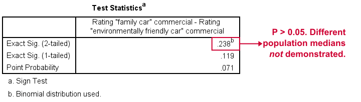
Exact Sig. (2-tailed) refers to our p-value of 0.24. This means there's a 24% chance of finding the observed difference if our null hypothesis is true. Our finding doesn't contradict our hypothesis is equal population medians.
In many cases the output will include “Asymp. Sig. (2-tailed)”, an approximate p-value based on the standard normal distribution.SPSS omits a continuity correction for calculating Z, which (slighly) biases p-values towards zero. It's not included now because our sample size n <= 25.

Reporting Our Sign Test Results

When reporting a sign test, include the entire table showing the signs and (possibly) ties. Although p-values can easily be calculated from it, we'll add something like “a sign test didn't show any difference between the two medians, exact binomial p (2-tailed) = 0.24.”

More on the P-Value

That's basically it. However, for those who are curious, we'll go into a little more detail now. First the p-value. Of our 18 cases, between 0 and 18 could have a plus (that is: rate ad1 higher than ad3). Our null hypothesis dictates that each case has a 0.5 probability of doing so, which is why the number of plusses follows the binomial sampling distribution shown below.

The most likely outcome is 9 plusses with a probability of roughly 0.175: if we'd draw 1,000 random samples instead of 1, we'd expect some 175 of those to result in 9 plusses. Roughly 12% of those samples should result in 6 or fewer plusses or 12 or more plusses. Reporting a 2-tailed p-value takes into account both tails (the areas in red) and thus results in p = 0.24 like we saw in the output.

SPSS Sign Test without a Sign Test

At this point you may see that the sign test is really equivalent to a binomial test on the variable holding our signs. This may come in handy if you want the exact p-value but only have the approximate p-value “Asymp. Sig. (2-tailed)” in your output. Our final syntax example shows how to get it done in 2 different ways.

Workaround for Exact P-Value

SPSS Median Test for 2 Independent Medians

The median test for independent medians tests if two or more populations have equal medians on some variable. That is, we're comparing 2(+) groups of cases on 1 variable at a time.

Rating Car Commercials

We'll demonstrate the median test on adratings.sav. This file holds data on 18 respondents who rated 3 different car commercials on attractiveness. A percent scale was used running from 0 (extremely unattractive commercial) through 100 (extremely attractive).

Median Test - Null Hypothesis

A marketeer wants to know if men rate the 3 commercials differently than women. After comparing the mean scores with a Mann-Whitney test, he also wants to know if the median scores are equal. A median test will answer the question by testing the null hypothesis that the population medians for men and women are equal for each rating variable.

Median Test - Assumptions

The median test makes only two assumptions:

• independent observations (or more precisely, independent and identically distributed variables);
• the test variable is ordinal or metric (that is, not nominal).

Quick Data Check

The adratings data don't hold any weird values or patterns. If you're analyzing any other data, make sure you always start with a data inspection. At the very least, run some histograms and check for missing values.

Median Test - Descriptives

Right, we're comparing 2 groups of cases on 3 rating variables. Let's first just take a look at the resulting 6 medians. The fastest way for doing so is running a basic MEANS command.

Result

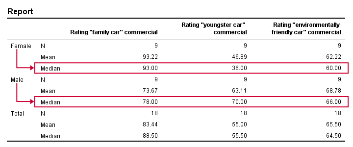
Very basically, the “family car” commercial was rated better by female respondents. Males were more attracted to the “youngster car” commercial. The “environmentally friendly car” commercial was rated roughly similarly by both genders -with regard to the medians anyway.
Now, keep in mind that this is just a small sample. If the population medians are exactly equal, then we'll probably find slightly different medians in our sample due to random sampling fluctuations. However, very different sample medians suggest that the population medians weren't equal after all. The median test tells us if equal population medians are credible, given our sample medians.

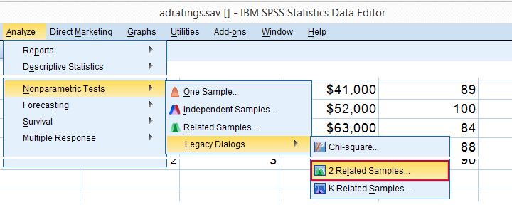
Median Test in SPSS

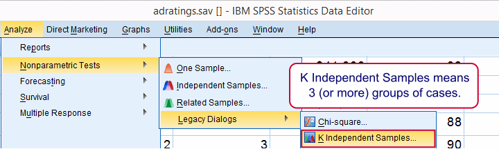
Usually, comparing 2 statistics is done with a different test than 3(+) statistics.For example, we use an independent samples t-test for 2 independent means and one-way ANOVA for 3(+) independent means. We use a paired samples t-test for 2 dependent means and repeated measures ANOVA for 3(+) dependent means. We use a McNemar test for 2 dependent proportions and a Cochran Q test for 3(+) dependent proportions. The median test is an exception because it's used for 2(+) independent medians. This is why we select K independent samples instead of 2 independent samples for comparing 2 medians.

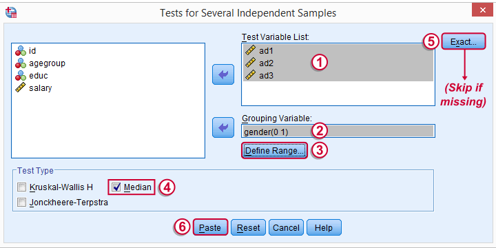
The Exact button may be absent, depending on your SPSS license. If it's present, fill it out as below.

SPSS Median Test Syntax

Completing these steps results in the syntax below (you'll have an extra line if you selected the exact test).

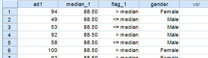
Median Test - How it Basically Works

Before inspecting our output, let's first take a look at how the test basically works for one variable.² The median test first computes a variable’s median, regardless of the groups we're comparing. Next, each case (row of data values) is flagged if its score > the pooled median. Finally, we'll see if scoring > the median is related to gender with a basic crosstab.You can pretty easily run these steps yourself with AGGREGATE, IF and CROSSTABS.

Median Test Output - Crosstabs

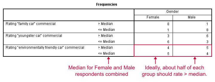
Note that these results are in line with the medians we ran earlier. The result for our “family car” commercial is particularly striking: 8 out of 9 respondents who score higher than the (pooled) median are female.

Median Test Output - Test Statistics

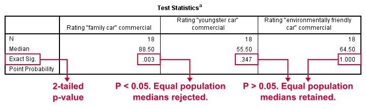
So are these normal outcomes if our population medians are equal across gender? For our first commercial, p = 0.003, indicating a chance of 3 in 1,000 of observing this outcome. Since p < 0.05, we conclude that the population medians are not equal for the “family car” commercial.
The other two commercials have p-values > 0.05 so these findings don't refute the null hypothesis of equal population medians.
So that's basically it for now. However, we would like to discuss the p-values into a little more detail for those who are interested.

Asymp. Sig.

In this example, we got exact p-values. However, when running this test on larger samples you may find “Asymp. Sig.” in your output. This is an approximate p-value based on the chi-square statistic and corresponding df (degrees of freedom). This approximation is sometimes used because the exact p-values are cumbersome to compute, especially for larger sample sizes.

Exact P-Values

So where do the exact p-values come from? How do they relate to the contingency tables we saw here? Well, the frequencies in the left upper cells follow a hypergeometric distribution.¹ Like so, the figure below shows where the second p-value of 0.347 comes from.

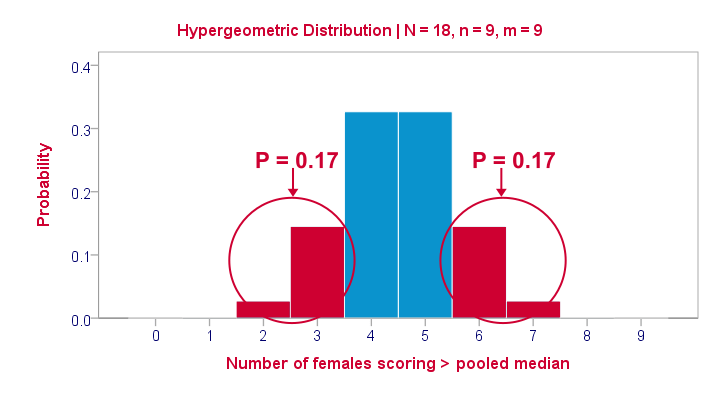
Under the null hypothesis -gender and scoring > the median are independent- the most likely outcome is 4 or 5, each with a probability around 0.33. The probability of 3 or fewer is roughly 0.17. This is our one-tailed p-value. Our two-tailed p-value takes into account the probability of 0.17 for finding a value of 6 or more because this would also contradict our null hypothesis.
The graph also illustrates why the two-tailed p-value for our third test is 1.000: the probability of 4 or fewer and 5 or more covers all possible outcomes. Regarding our first test, the probability of 1 or fewer and 8 or more is close to zero (precisely: 0.003).

Median Test with CROSSTABS

Right, so the previous figure explains how exact p-values are based on the hypergeometric distribution. This procedure is known as Fisher’s exact test and you may have seen it in SPSS CROSSTABS output when running a chi-square independence test. And -indeed- you can obtain the exact p-values for our independent medians test from CROSSTABS too. In fact, you can even compute them as a new variable in your data with compute p2 = 2* cdf.hyper(3,18,9,9).
execute. which returns 0.347, the p-value for our second commercial.

Thanks for reading!

References

1. Siegel, S. & Castellan, N.J. (1989). Nonparametric Statistics for the Behavioral Sciences (2nd ed.). Singapore: McGraw-Hill.
2. Van den Brink, W.P. & Koele, P. (2002). Statistiek, deel 3 [Statistics, part 3]. Amsterdam: Boom.

SPSS Friedman Test Tutorial

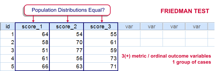
For testing if 3 or more variables have identical population means, our first option is a repeated measures ANOVA. This requires our data to meet some assumptions -like normally distributed variables. If such assumptions aren't met, then our second option is the Friedman test: a nonparametric alternative for a repeated-measures ANOVA.
Strictly, the Friedman test can be used on quantitative or ordinal variables but ties may be an issue in the latter case.

The Friedman Test - How Does it Work?

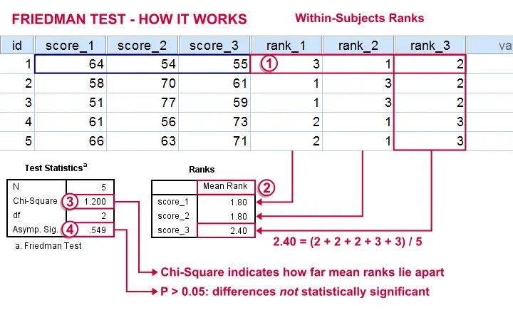
The original variables are ranked within cases.
The mean ranks over cases are computed. If the original variables have similar distributions, then the mean ranks should be roughly equal.
The test-statistic, Chi-Square is like a variance over the mean ranks: it's 0 when the mean ranks are exactly equal and becomes larger as they lie further apart.In ANOVA we find a similar concept: the “mean square between” is basically the variance between sample means. This is explained in ANOVA - What Is It?.
Asymp. Sig. is our p-value. It's the probability of finding our sample differences if the population distributions are equal. The differences in our sample have a large (0.55 or 55%) chance of occurring. They don't contradict our hypothesis of equal population distributions.

The Friedman Test in SPSS

Let's first take a look at our data in adratings.sav, part of which are shown below. The data contain 18 respondents who rated 3 commercials for cars on a percent (0% through 100% attractive) scale.

We'd like to know which commercial performs best in the population. So we'll first see if the mean ratings in our sample are different. If so, the next question is if they're different enough to conclude that the same holds for our population at large. That is, our null hypothesis is that the population distributions of our 3 rating variables are identical.

Quick Data Check

Inspecting the histograms of our rating variables will give us a lot of insight into our data with minimal effort. We'll create them by running the syntax below.

Result

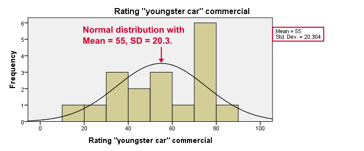
Most importantly, our data look plausible: we don't see any outrageous values or patterns. Note that the mean ratings are pretty different: 83, 55 and 66. Every histogram is based on all 18 cases so there's no missing values to worry about.
Now, by superimposing normal curves over our histograms, we do see that our variables are not quite normally distributed as required for repeated measures ANOVA. This isn't a serious problem for larger sample sizes (say, n > 25 or so) but we've only 18 cases now. We'll therefore play it safe and use a Friedman test instead.

Running a Friedman Test in SPSS

K Related Samples means that we'll compare 3 or more variables measured on the same respondents. This is similar to “within-subjects effect” we find in repeated measures ANOVA.

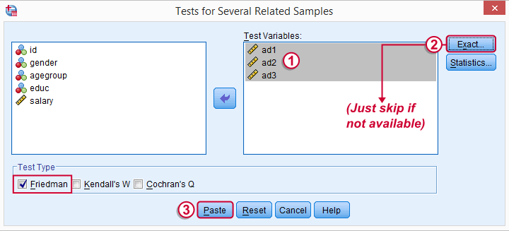
Depending on your SPSS license, you may or may not have the Exact button. If you do, fill it out as below and otherwise just skip it.

SPSS Friedman Test - Syntax

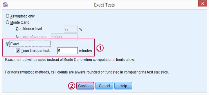
Following these steps results in the syntax below (you'll have 1 extra line if you selected the exact statistics). Let's run it.

SPSS Friedman Test - Output

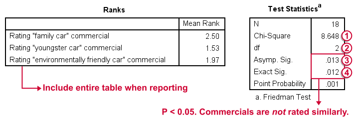
First note that the mean ranks differ quite a lot in favor of the first (“Family Car”) commercial. Unsurprisingly, the mean ranks have the same order as the means we saw in our histogram.
Chi-Square (more correctly referred to as Friedman’s Q) is our test statistic. It basically summarizes how differently our commercials were rated in a single number.
df are the degrees of freedom associated with our test statistic. It's equal to the number of variables we compare - 1. In our example, 3 variables - 1 = 2 degrees of freedom.
Asymp. Sig. is an approximate p-value. Since p < 0.05, we refute the null hypothesis of equal population distributions.“Asymp” is short for “asymptotic”: the more our sample size increases towards infinity, the more the sampling distribution of Friedman’s Q becomes similar to a χ² distribution. Reversely, this χ² approximation is less precise for smaller samples.
Exact Sig. is the exact p-value. If available, we prefer it over the asymptotic p-value, especially for smaller sample sizes.If there's an exact p-value, then why would anybody ever use an approximate p-value? The basic reason is that the exact p-value requires very heavy computations, especially for larger sample sizes. Modern computers deal with this pretty well but this hasn't always been the case.

Friedman Test - Reporting

As indicated previously, we'll include the entire table of mean ranks in our report. This tells you which commercial was rated best versus worst. Furthermore, we could write something like “a Friedman test indicated that our commercials were rated differently, χ²(2) = 8.65, p = 0.013.“ We personally disagree with this reporting guideline. We feel Friedman’s Q should be called “Friedman’s Q” instead of “χ²”. The latter is merely an approximation that may or may not be involved when calculating the p-value. Furthermore, this approximation becomes less accurate as the sample size decreases. Friedman’s Q is by no means the same thing as χ² so we feel they should not be used interchangeably.

So much for the Friedman test in SPSS. I hope you found this tutorial useful. Thanks for reading.

SPSS Wilcoxon Signed-Ranks Test – Simple Example

For comparing two metric variables measured on one group of cases, our first choice is the paired-samples t-test. This requires the difference scores to be normally distributed in our population. If this assumption isn't met, we can use Wilcoxon S-R test instead. It can also be used on ordinal variables -although ties may be a real issue for Likert items.
Don't abbreviate “Wilcoxon S-R test” to simply “Wilcoxon test” like SPSS does: there's a second “Wilcoxon test” which is also known as the Mann-Whitney test for two independent samples.

Wilcoxon Signed-Ranks Test - How It Basically Works

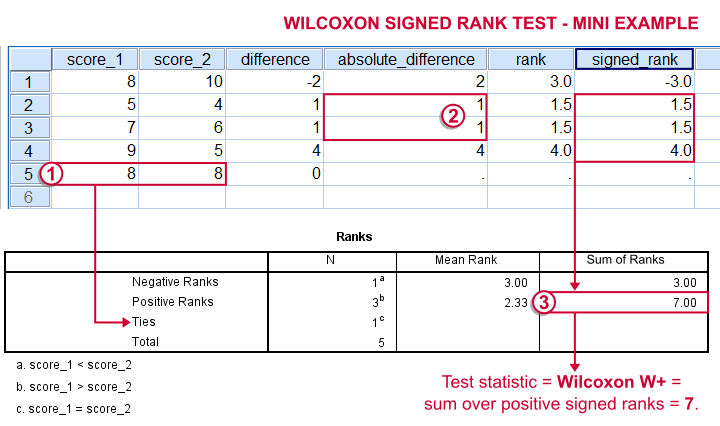
1. For each case calculate the difference between score_1 and score_2. Ties (cases whose two values are equal) are excluded from this test altogether.
2. Calculate the absolute difference for each case.
3. Rank the absolute differences over cases. Use mean ranks for ties (different cases with equal absolute difference scores).
4. Create signed ranks by applying the signs (plus or minus) of the differences to the ranks.
5. Compute the test statistic Wilcoxon W+, which is the sum over positive signed ranks. If score_1 and score_2 really have similar population distributions, then W+ should be neither very small nor very large.
6. Calculate the p-value for W+ from its exact sampling distribution or approximate it by a standard normal distribution.

So much for the theory. We'll now run Wilcoxon S-R test in SPSS on some real world data.

Adratings Data - Brief Description.

A car manufacturer had 18 respondents rate 3 different commercials for one of their cars. They first want to know which commercial is rated best by all respondents. These data -part of which are shown below- are in adratings.sav.

Quick Data Check

Our current focus is limited to the 3 rating variables, ad1 through ad3. Let's first make sure we've an idea what they basically look like before carrying on. We'll inspect their histograms by running the syntax below.

Basic Histograms Syntax

Histograms - Results

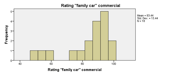
First and foremost, our 3 histograms don't show any weird values or patterns so our data look credible and there's no need for specifying any user missing values.
Let's also take a look at the descriptive statistics in our histograms. Each variable has n = 18 respondents so there aren't any missing values at all. Note that ad2 (the “Youngster car commercial”) has a very low average rating of only 55. It's decided to drop this commercial from the analysis and test if ad1 and ad3 have equal mean ratings.

Difference Scores

Let's now compute and inspect the difference scores between ad1 and ad3 with the syntax below.

Result

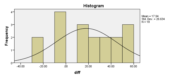
Our first choice for comparing these variables would be a paired samples t-test. This requires the difference scores to be normally distributed in our population but our sample suggests otherwise. This isn't a problem for larger samples sizes (say, n > 25) but we've only 18 respondents in our data.For larger sample sizes, the central limit theorem ensures that the sampling distribution of the mean will be normal, regardless of the population distribution of a variable. Fortunately, Wilcoxon S-R test was developed for precisely this scenario: not meeting the assumptions of a paired-samples t-test. Only now can we really formulate our null hypothesis: the population distributions for ad1 and ad3 are identical. If this is true, then these distributions will be slightly different in a small sample like our data at hand. However, if our sample shows very different distributions, then our hypothesis of equal population distributions will no longer be tenable.

Wilcoxon S-R test in SPSS - Menu

Now that we've a basic idea what our data look like, let's run our test. The screenshots below guide you through.

2 Related Samples refers to comparing 2 variables measured on the same respondents. This is similar to “paired samples” or “within-subjects” effects in repeated measures ANOVA.

Optionally, reverse the variable order so you have the highest scores (ad1 in our data) under Variable2.
“Wilcoxon” refers to Wilcoxon S-R test here. This is a different test than Wilcoxon independent samples test (also know as Mann-Whitney test).
Exact may or may not be present, depending on your SPSS license. If you do have it, we propose you fill it out as below.

Wilcoxon S-R test in SPSS - Syntax

Following these steps results in the syntax below (you'll have one extra line if you requested exact statistics).

Wilcoxon S-R Test - Ranks Table Ouput

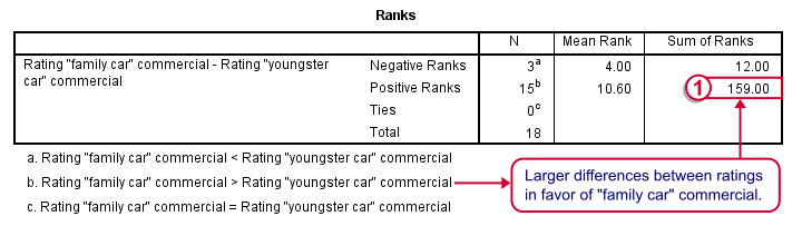
Let's first stare at this table and its footnotes for a minute and decipher what it really says. Right. Now, if ad1 and ad3 have similar population distributions, then the signs (plus and minus) should be distributed roughly evenly over ranks. If you find this hard to grasp -like most people- take another look at this diagram.
This implies that the sum of positive ranks should be close to the sum of negative ranks. This number (159 in our example) is our test statistic and known as Wilcoxon W+.
Our table shows a very different pattern: the sum of positive ranks (indicating that the “Family car” was rated better) is way larger than the sum of negative ranks. Can we still believe our 2 commerials are rated similarly?

Wilcoxon S-R Test - Test Statistics Ouput

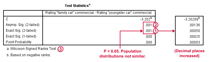
Oddly, our ”Test Statistics“ table includes everything except for our actual test statistic, the aforementioned W+.
We prefer reporting Exact Sig. (2-tailed). Its value of 0.001 means that the probability is roughly 1 in 1,000 of finding the large sample difference we did if our variables really have similar population distributions.
If our output doesn't include the exact p-value, we'll report Asymp. Sig. (2-tailed) instead, which is also 0.001. This approximate p-value is based on the standard normal distribution (hence the “Z” right on top of it).“Asymp” is short for asymptotic. It means that as the sample size approaches infinity, the sampling distribution of W+ becomes identical to a normal distribution. Or more practically: this normal approximation is more accurate for larger sample sizes.
It's comforting to see that both p-values are 0.001. Apparently, the normal approximation is accurate. However, if we increase the decimal places, we see that it's almost three times larger than the exact p-value.A nice tool for doing so is downloadable from Set Decimals for Output Tables Tool.
The reason for having two p-values is that the exact p-value can be computationally heavy, especially for larger sample sizes.

How to Report Wilcoxon Signed-Ranks Test?

The official way for reporting these results is as follows: “A Wilcoxon Signed-Ranks test indicated that the “Family car” commercial (mean rank = 10.6) was rated more favorably than the “Youngster car” commercial (mean rank = 4.0), Z = -3.2, p = 0.001.” We think this guideline is poor for smaller sample sizes. In this case, the Z-approximation may be unnecessary and inaccurate and the exact p-value is to be preferred.

I hope this tutorial has been helpful in understanding and using Wilcoxon Signed-Ranks test in SPSS. Please let me know by leaving a comment below. Thanks!

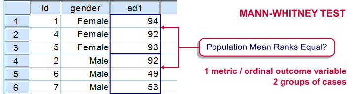
SPSS Mann-Whitney Test Tutorial

Introduction & Practice Data File

The Mann-Whitney test is an alternative for the independent samples t-test when the assumptions required by the latter aren't met by the data. The most common scenario is testing a non normally distributed outcome variable in a small sample (say, n < 25).Non normality isn't a serious issue in larger samples due to the central limit theorem.

The Mann-Whitney test is also known as the Wilcoxon test for independent samples -which shouldn't be confused with the Wilcoxon signed-ranks test for related samples.

Research Question

We'll use adratings.sav during this tutorial, a screenshot of which is shown above. These data contain the ratings of 3 car commercials by 18 respondents, balanced over gender and age category. Our research question is whether men and women judge our commercials similarly. For each commercial separately, our null hypothesis is: “the mean ratings of men and women are equal.”

Quick Data Check - Split Histograms

Before running any significance tests, let's first just inspect what our data look like in the first place. A great way for doing so is running some histograms. Since we're interested in differences between male and female respondents, let's split our histograms by gender. The screenshots below guide you through.

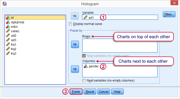
Split Histograms - Syntax

Using the menu results in the first block of syntax below. We copy-paste it twice, replace the variable name and run it.

Split Histograms - Results

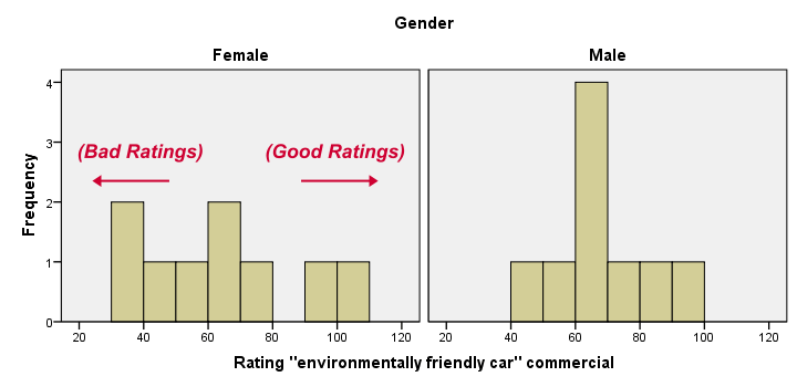
Most importantly, all results look plausible; we don't see any unusual values or patterns. Second, our outcome variables don't seem to be normally distributed and we've a total sample size of only n = 18. This argues against using a t-test for these data.
Finally, by taking a good look at the split histograms, you can already see which commercials are rated more favorably by male versus female respondents. But even if they're rated perfectly similarly by large populations of men and women, we'll still see some differences in small samples. Large sample differences, however, are unlikely if the null hypothesis -equal population means- is really true. We'll now find out if our sample differences are large enough for refuting this hypothesis.

SPSS Mann-Whitney Test - Menu

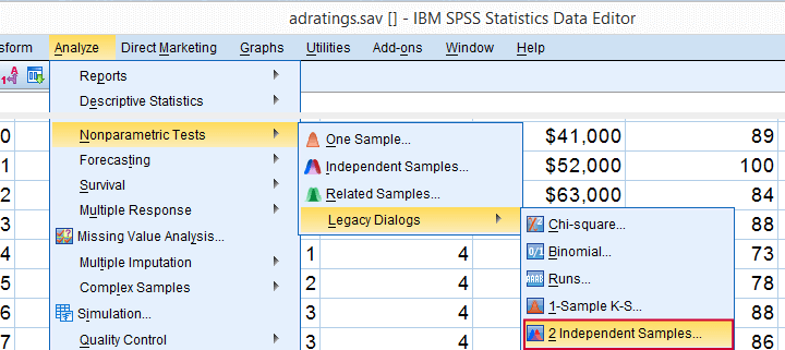
Depending on your SPSS license, you may or may not have the Exact submenu available. If you don't have it, just skip the step below.

SPSS Mann-Whitney Test - Syntax

Note: selecting Exact results in an extra line of syntax (omitted below).

SPSS Mann-Whitney Test - Output Descriptive Statistics

The Mann-Whitney test basically replaces all scores with their rank numbers: 1, 2, 3 through 18 for 18 cases. Higher scores get higher rank numbers. If our grouping variable (gender) doesn't affect our ratings, then the mean ranks should be roughly equal for men and women.

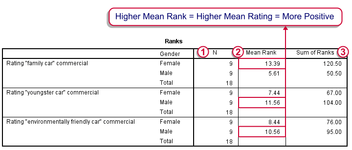
Our first commercial (“Family car”) shows the largest difference in mean ranks between male and female respondents: females seem much more enthusiastic about it. The reverse pattern -but much weaker- is observed for the other two commercials.

SPSS Mann-Whitney Test - Output Significance Tests

Some of the output shown below may be absent depending on your SPSS license and the sample size: for n = 40 or fewer cases, you'll always get some exact results.

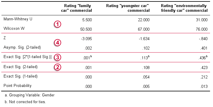
Mann-Whitney U and Wilcoxon W are our test statistics; they summarize the difference in mean rank numbers in a single number.Note that Wilcoxon W corresponds to the smallest sum of rank numbers from the previous table.
We prefer reporting Exact Sig. (2-tailed): the exact p-value corrected for ties.
Second best is Exact Sig. [2*(1-tailed Sig.)], the exact p-value but not corrected for ties.
For larger sample sizes, our test statistics are roughly normally distributed. An approximate (or “Asymptotic”) p-value is based on the standard normal distribution. The z-score and p-value reported by SPSS are calculated without applying the necessary continuity correction, resulting in some (minor) inaccuracy.

SPSS Mann-Whitney Test - Conclusions

Like we just saw, SPSS Mann-Whitney test output may include up to 3 different 2-sided p-values. Fortunately, they all lead to the same conclusion if we follow the convention of rejecting the null hypothesis if p < 0.05: Women rated the “Family Car” commercial more favorably than men (p = 0.001). The other two commercials didn't show a gender difference (p > 0.10). The p-value of 0.001 indicates a probability of 1 in 1,000: if the populations of men and women rate this commercial similarly, then we've a 1 in 1,000 chance of finding the large difference we observe in our sample. Presumably, the populations of men and women don't rate it similarly after all.

So that's about it. Thanks for reading and feel free to leave a comment below!

Binomial Test – Simple Tutorial

For running a binomial test in SPSS, see SPSS Binomial Test.

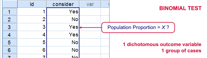
A binomial test examines if some
population proportion is likely to be x. For example, is 50% -a proportion of 0.50- of the entire Dutch population familiar with my brand? We asked a simple random sample of N = 10 people if they are. Only 2 of those -a proportion of 0.2- or 20% know my brand. Does this sample proportion of 0.2 mean that the population proportion is not 0.5? Or is 2 out of 10 a pretty normal outcome if 50% of my population really does know my brand?
The binomial test is the simplest statistical test there is. Understanding how it works is pretty easy and will help you understand other statistical significance tests more easily too. So how does it work?

Binomial Test - Basic Idea

If the population proportion really is 0.5, we can find a sample proportion of 0.2. However, if the population proportion is only 0.1 (only 10% of all Dutch adults know the brand), then we may also find a sample proportion of 0.2. Or 0.9. Or basically any number between 0 and 1. The figure below illustrates the basic problem -I mean challenge- here.

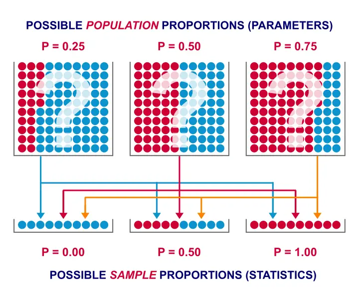Will the real population proportion please stand up now??

So how can we conclude anything at all about our population based on just a sample? Well, we first make an initial guess about the population proportion which we call the null hypothesis: a population proportion of 0.5 knows my brand.
Given this hypothesis, many sample proportions are possible. However, some outcomes are extremely unlikely or almost impossible. If we do find an outcome that's almost impossible given some hypothesis, then the hypothesis was probably wrong: we conclude that the population proportion wasn't x after all.
So that's how we draw population conclusions based on sample outcomes. Basically all statistical tests follow this line of reasoning. The basic question for now is: what's the probability of finding 2 successes in a sample of 10 if the population proportion is 0.5?

Binomial Test Assumptions

First off, we need to assume independent observations. This basically means that the answer given by any respondent must be independent of the answer given by any other respondent. This assumption (required by almost all statistical tests) has been met by our data.

Binomial Distribution - Formula

If 50% of some population knows my brand and I ask 10 people, then my sample could hold anything between 0 and 10 successes. Each of these 11 possible outcomes and their associated probabilities are an example of a binomial distribution, which is defined as $$P(B = k) = \binom{n}{k} p^k (1 - p)^{n - k}$$ where

• \(n\) is the number of trials (sample size);
• \(k\) is the number of successes;
• \(p\) is the probability of success for a single trial or the (hypothesized) population proportion.

Note that \(\binom{n}{k}\) is a shorthand for \(\frac{n!}{k!(n - k)!}\) where \(!\) indicates a factorial.

For practical purposes, we get our probabilities straight from Google Sheets (it uses the aforementioned formula under the hood but it doesn't bother us with it).

Binomial Distribution - Chart

Right, so we got the probabilities for our 11 possible outcomes (0 through 10 successes) and visualized them below.

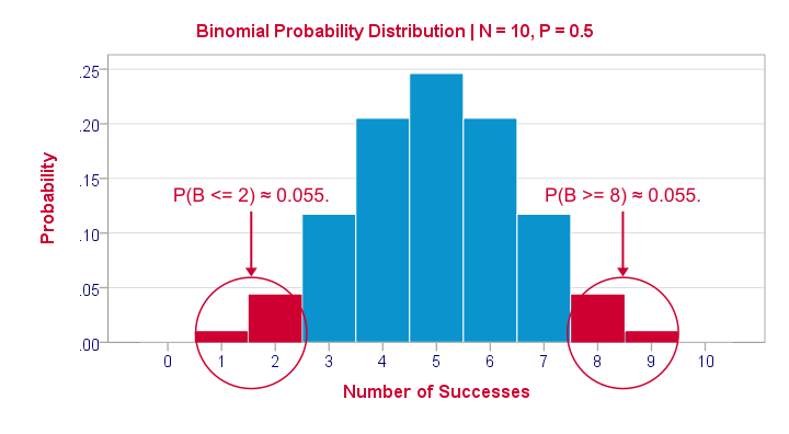
If a population proportion is 0.5 and we sample 10 observations, the most likely outcome is 5 successes: P(B = 5) ≈ 0.24. Either 4 or 6 successes are also likely outcomes (P ≈ 0.2 for each).
The probability of finding 2 or fewer successes -like we did- is 0.055. This is our one-sided p-value.
Now, very low or very high numbers of successes are both unlikely outcomes and should both cast doubt on our null hypothesis. We therefore take into account the p-value for the opposite outcome -8 or more successes- which is another 0.055. Like so, we find a 2-sided p-value of 0.11. If we would draw 1,000 samples instead of just 1, then some 11% of those should result in 2(-) or 8(+) successes when the population proportion is 0.5. Our sample outcome should occur in a reasonable percentage of samples. And since 11% is not very unlikely, our sample does not refute our hypothesis that 50% of our population knows our brand.

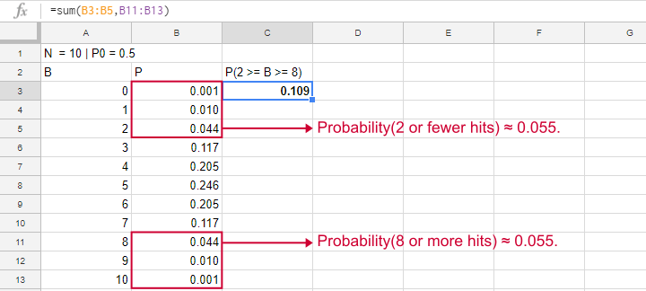
Binomial Test - Google Sheets

We ran our example in this simple Google Sheet. It's accessible to anybody so feel free to take a look at it.

Binomial Test - SPSS

Perhaps the easiest way to run a binomial test is in SPSS - for a nice tutorial, try SPSS Binomial Test. The figure below shows the output for our current example. It obviously returns the same p-value of 0.109 as our Google Sheet.

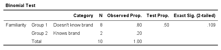
Note that SPSS refers to p as “Exact Sig. (2-tailed)”. Is there a non exact p-value too then? Well, sort of. Let's see how that works.

Binomial Test or Z Test?

Let's take another look at the binomial probability distribution we saw earlier. It kinda resembles a normal distribution. Not convinced? Take a look at the binomial distribution below.

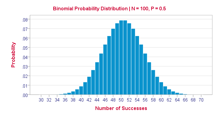
For a sample of N = 100, our binomial distribution is virtually identical to a normal distribution. This is caused by the central limit theorem. A consequence is that -for a larger sample size- a z-test for one proportion (using a standard normal distribution) will yield almost identical p-values as our binomial test (using a binomial distribution).

But why would we prefer a z-test over a binomial test?

• We can always use a 2-sided z-test. However, a binomial test is always 1-sided unless P₀ = 0.5.
• A z-test allows us to compute a confidence interval for our sample proportion.
• We can easily estimate statistical power for a z-test but not for a binomial test.
• A z-test is computationally less heavy, especially for larger sample sizes.I suspect that most software actually reports a z-test as if it were a binomial test for larger sample sizes.

So when can we use a z-test instead of a binomial test? A rule of thumb is that P₀*n and (1 - P₀)*n must both be > 5, where P₀ denotes the hypothesized population proportion and n the sample size.

So that's about it regarding the binomial test. I hope you found this tutorial helpful. Thanks for reading!

How to Run a Kruskal-Wallis Test in SPSS?

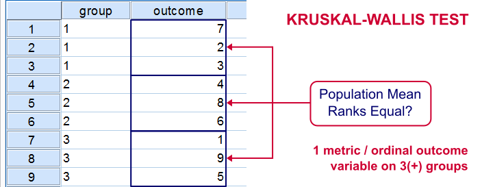
The Kruskal-Wallis test is an alternative for a one-way ANOVA if the assumptions of the latter are violated. We'll show in a minute why that's the case with creatine.sav, the data we'll use in this tutorial. But let's first take a quick look at what's in the data anyway.

Quick Data Description

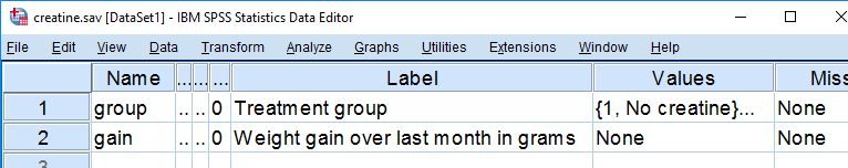
Our data contain the result of a small experiment regarding creatine, a supplement that's popular among body builders. These were divided into 3 groups: some didn't take any creatine, others took it in the morning and still others took it in the evening. After doing so for a month, their weight gains were measured. The basic research question is does the average weight gain depend on
the creatine condition to which people were assigned? That is, we'll test if three means -each calculated on a different group of people- are equal. The most likely test for this scenario is a one-way ANOVA but using it requires some assumptions. Some basic checks will tell us that these assumptions aren't satisfied by our data at hand.

Data Check 1 - Histogram

A very efficient data check is to run histograms on all metric variables. The fastest way for doing so is by running the syntax below.

Histogram Result

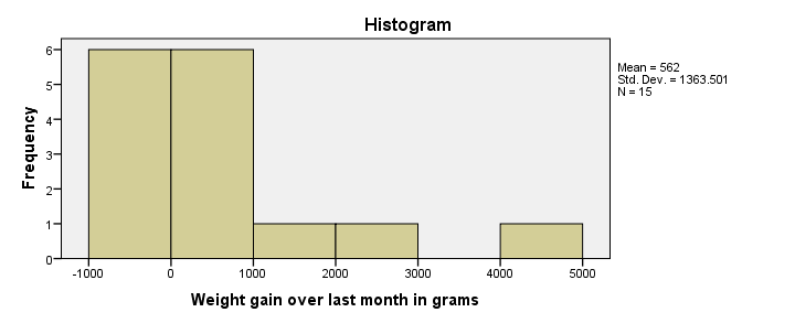
First, our histogram looks plausible with all weight gains between -1 and +5 kilos, which are reasonable outcomes over one month. However, our outcome variable is not normally distributed as required for ANOVA. This isn't an issue for larger sample sizes of, say, at least 30 people in each group. The reason for this is the central limit theorem. It basically states that for reasonable sample sizes the sampling distribution for means and sums are always normally distributed regardless of a variable’s original distribution. However, for our tiny sample at hand, this does pose a real problem.

Data Check 2 - Descriptives per Group

Right, now after making sure the results for weight gain look credible, let's see if our 3 groups actually have different means. The fastest way to do so is a simple MEANS command as shown below.

SPSS MEANS Output

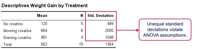
First, note that our evening creatine group (4 participants) gained an average of 961 grams as opposed to 120 grams for “no creatine”. This suggests that creatine does make a real difference.
But don't overlook the standard deviations for our groups: they are very different but ANOVA requires them to be equal.The assumption of equal population standard deviations for all groups is known as homoscedasticity. This is a second violation of the ANOVA assumptions.

Kruskal-Wallis Test

So what should we do now? We'd like to use an ANOVA but our data seriously violates its assumptions. Well, a test that was designed for precisely this situation is the Kruskal-Wallis test which doesn't require these assumptions. It basically replaces the weight gain scores with their rank numbers and tests whether these are equal over groups. We'll run it by following the screenshots below.

Running a Kruskal-Wallis Test in SPSS

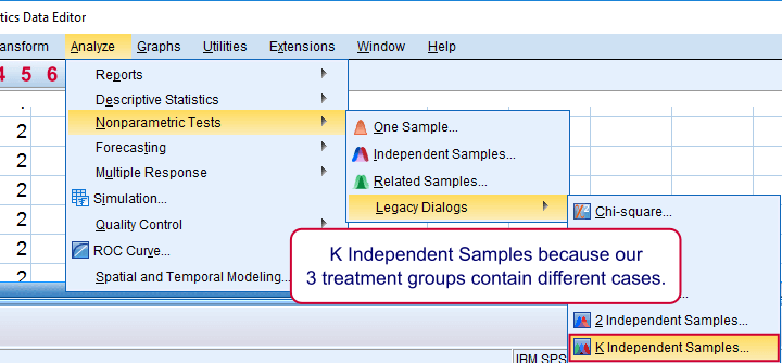
We use K Independent Samples if we compare 3 or more groups of cases. They are “independent” because our groups don't overlap (each case belongs to only one creatine condition).

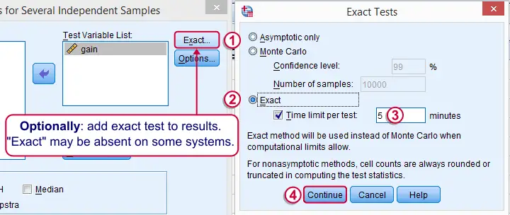
Depending on your license, your SPSS version may or may have the Exact option shown below. It's fine to skip this step otherwise.

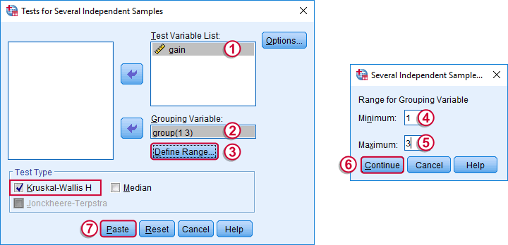
SPSS Kruskal-Wallis Test Syntax

Following the previous screenshots results in the syntax below. We'll run it and explain the output.

SPSS Kruskal-Wallis Test Output

We'll skip the “RANKS” table and head over to the “Test Statistics” shown below.

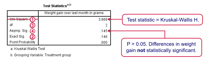
Our test statistic -incorrectly labeled as “Chi-Square” by SPSS- is known as Kruskal-Wallis H. A larger value indicates larger differences between the groups we're comparing. For our data it's roughly 3.87. We need to know its sampling distribution for evaluating whether this is unusually large.
Exact Sig. uses the exact (but very complex) sampling distribution of H. However, it turns out that if each group contains 4 or more cases, this exact sampling distribution is almost identical to the (much simpler) chi-square distribution.
We therefore usually approximate the p-value with a chi-square distribution. If we compare k groups, we have k - 1 degrees of freedom, denoted by df in our output.
Asymp. Sig. is the p-value based on our chi-square approximation. The value of 0.145 basically means there's a 14.5% chance of finding our sample results if creatine doesn't have any effect in the population at large. So if creatine does nothing whatsoever, we have a fair (14.5%) chance of finding such minor weight gain differences just because of random sampling. If p > 0.05, we usually conclude that our differences are not statistically significant.
Note that our exact p-value is 0.146 whereas the approximate p-value is 0.145. This supports the claim that H is almost perfectly chi-square distributed.

Kruskal-Wallis Test - Reporting

The official way for reporting our test results includes our chi-square value, df and p as in “this study did not demonstrate any effect from creatine,
H(2) = 3.87, p = 0.15.”

So that's it for now. I hope you found this tutorial helpful. Please let me know by leaving a comment below. Thanks!