SPSS Label Cleaning Tool
We sometimes receive data files with annoying prefixes or suffixes in variable and/or value labels. This tutorial presents a simple tool for removing these and some other “cleaning” operations.
- Prerequisites and Installation
- Example I - Text Replacement over Variable and Value Labels
- Example II - Remove Suffix from Variable Labels
- Example III - Remove Prefix from Value Labels
Example Data File
All examples in this tutorial use dirty-labels.sav. As shown below, its labels are far from ideal.
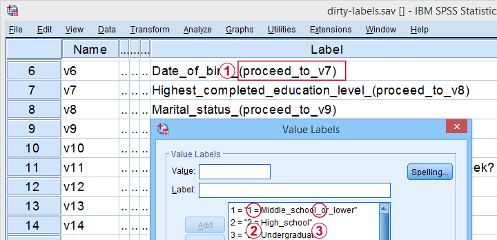
 Some variable labels have suffixes that are irrelevant to the final data.
 All value labels are prefixed by the values that represent them.
 Variable and value labels have underscores instead of spaces.
Our tool deals with precisely such issues. Let's try it.
Prerequisites and Installation
First off, this tool requires SPSS version 24 or higher. Next, the SPSS Python 3 essentials must be installed, which is normally the case with recent SPSS versions.
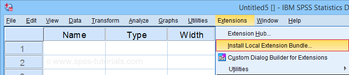
Next, click SPSS_TUTORIALS_CLEAN_LABELS.spe for downloading our tool. You can install it by dragging & dropping it into a data editor window. Alternatively, navigate to
![]() as shown below.
as shown below.
In the dialog that opens, navigate to the downloaded .spe file and select it. SPSS now throws a message that “The extension was successfully installed under Transform - SPSS tutorials - Clean Labels”.
Example I - Text Replacement over Variable and Value Labels
Let's first replace all underscores by spaces in both variable and value labels. We'll open
![]() and fill out the dialog as shown below.
and fill out the dialog as shown below.
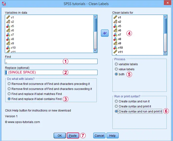
Completing these steps results in the syntax below. Let's run it.
SPSS TUTORIALS CLEAN_LABELS VARIABLES=v1 v2 v5 v6 v7 v8 v9 v10 v11 v12 v13 v14 v15 v16 v17 v18 v19
v20 v21 v22 FIND='_' REPLACEBY=' '
/OPTIONS OPERATION=FIREPCONT PROCESS=BOTH ACTION=BOTH.
Results
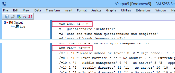
First note that all underscores were replaced by spaces in all variable and value labels. This was done by creating and running
- VARIABLE LABELS and
- ADD VALUE LABELS
commands. We chose to have these commands printed to our output window as shown below.
SPSS already ran this syntax but you can also copy-paste it into a syntax window. Like so, the adjustments can be replicated on any SPSS version with or without our tool installed. If there's a lot of syntax, consider moving it into a separate file and running it with INSERT.
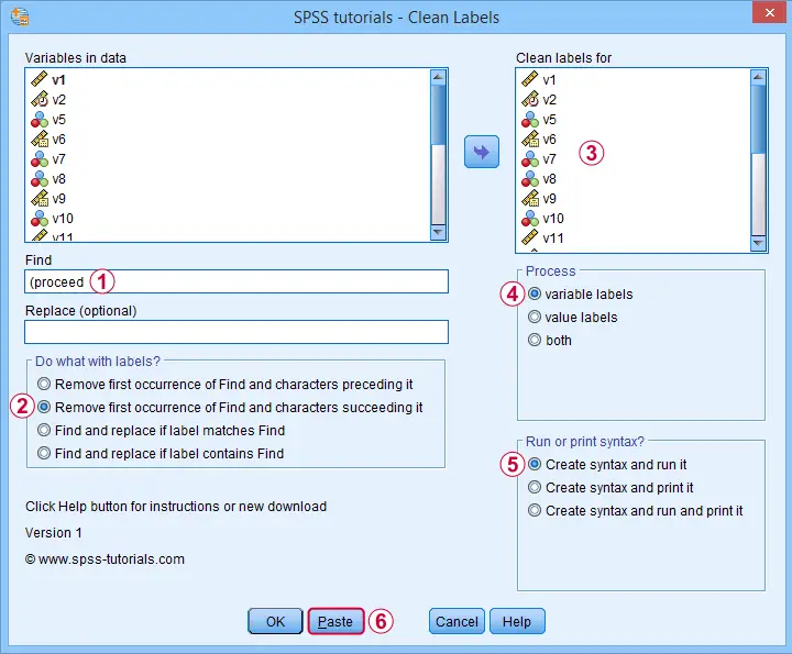
Example II - Remove Suffix from Variable Labels
Some variable labels end with “ (proceed to question...” We'll remove these suffixes because they don't convey any interesting information and merely clutter up our output tables and charts.
Again, we start off at
![]() and fill out the dialog as shown below.
and fill out the dialog as shown below.
Quick tip: you can shorten the resulting syntax by using
- TO for specifying a range of variables such as V5 TO V1;
- ALL for specifying all variables in the active dataset.
We did just that in the syntax below.
SPSS TUTORIALS CLEAN_LABELS VARIABLES=all FIND=' (proceed' REPLACEBY=' '
/OPTIONS OPERATION=FIOCSUC PROCESS=VARLABS ACTION=RUN.
Note that running this syntax removes “ (proceed to” and all characters that follow this expression from all variable labels.
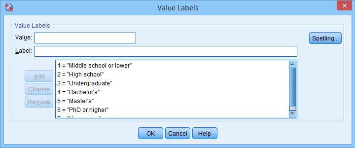
Example III - Remove Prefix from Value Labels
Another issue we sometimes encounter are value labels being prefixed with the values representing them as shown below.
Removing “= ” (mind the space) and all characters preceding it from all value labels fixes the problem. The syntax below -created from
![]() -
does just that.
-
does just that.
SPSS TUTORIALS CLEAN_LABELS VARIABLES=all FIND='= ' REPLACEBY=' '
/OPTIONS OPERATION=FIOCPRE PROCESS=VALLABS ACTION=RUN.
Result
After our third and final example, all value and variable labels are nice, short can clean.
So that'll wrap up the examples of our label cleaning tool.
Final Notes
I hope you'll find our tool as helpful as we do. This first version performs 4 cleaning operations that we recently needed for our daily work. We'll probably build in some more options when we (or you?) need them.
So if you've any suggestions or other remarks, please throw us a comment below. Other than that,
thanks for reading!
SPSS Mean Centering and Interaction Tool
Also see SPSS Moderation Regression Tutorial.
- Regression with Moderation Effect
- Downloading and Installing the Mean Centering Tool
- Using the Mean Centering Tool
- Mean Centering Tool - Results
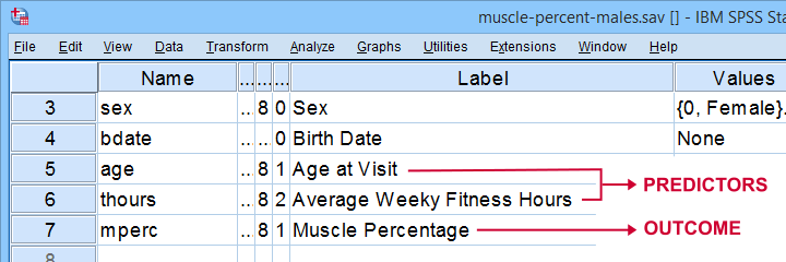
A sports doctor wants to know if and how training and age relate to body muscle percentage. His data on 243 male patients are in muscle-percent-males.sav, part of which is shown below.
Regression with Moderation Effect
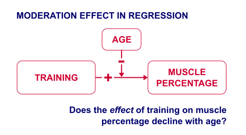
The basic way to go with these data is to run multiple regression with age and training hours as predictors. However, our doctor expects a moderation interaction effect between age and training. Precisely, he believes that the effect of training on muscle percentage diminishes with age. The diagram below illustrates the basic idea.
The moderation effect can be tested by creating a new variable that represents this interaction effect. We'll do just that in 3 steps:
- mean center both predictors: subtract the variable means from all individual scores. This results in centered predictors having zero means.
- compute the interaction predictor as the product of the mean centered predictors;
- run a multiple regression analysis with 3 predictors: the mean centered predictors and the interaction predictor.
Steps 1 and 2 can be done with basic syntax as covered in How to Mean Center Predictors in SPSS? However, we'll present a simple tool below that does these steps for you.
Downloading and Installing the Mean Centering Tool
First off, you need SPSS with the SPSS-Python-Essentials for installing this tool. The tool is downloadable from SPSS_TUTORIALS_MEAN_CENTER.spe.
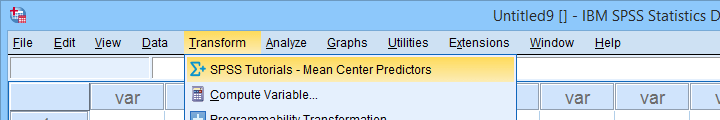
After downloading it, open SPSS and navigate to
![]() as shown below.
as shown below.
For older SPSS versions, try
![]() You may need to run SPSS as an administrator (by right-clicking its desktop shortcut) in order to install any tools.
You may need to run SPSS as an administrator (by right-clicking its desktop shortcut) in order to install any tools.
Using the Mean Centering Tool
First open some data such as muscle-percent-males.sav. After installing the mean centering tool, you'll find it in the menu.
This opens a dialog as shown below. Note that string variables don't show up here: these need to be converted to numeric variable before they can be mean centered.
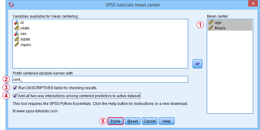
 Variable names for the centered predictors consist of a prefix + the original variable names. In this example, mean centered age and thours will be named cent_age and cent_thours.
 Optionally, create new variables holding all 2-way interaction effects among the centered predictors. For 2 predictors, this results in only 1 interaction predictor.
 Clicking results in the syntax below. Let's run it.
SPSS_TUTORIALS_MEAN_CENTER VARIABLES = "age thours"
/OPTIONS PREFIX = cent_ CHECKTABLE INTERACTIONS.
Mean Centering Tool - Results
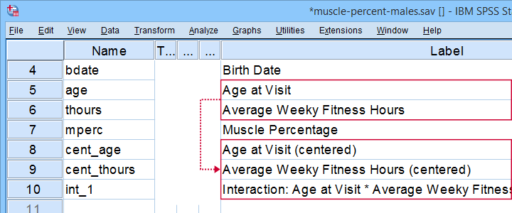
In variable view, note that 3 new variables have been created (and labeled). Precisely these 3 variables should be entered as predictors into our regression model.
If a checktable was requested, you'll find a basic Descriptive Statistics table in the output window.
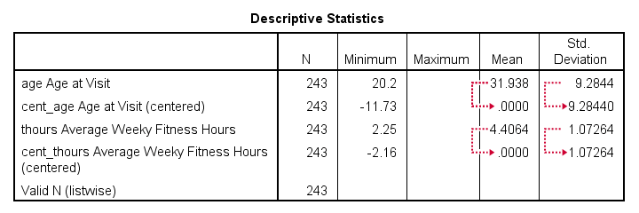
Note that the mean centered predictors have exactly zero means. Their standard deviations, however, are left unaltered by the mean centering -which is precisely how this procedure differs from computing z-scores.
Right, so that'll do for our mean centering tool. We'll cover a regression analysis with a moderation interaction effect in 1 or 2 weeks or so.
Thanks for reading!
SPSS – Create Dummy Variables Tool
Categorical variables can't readily be used as predictors in multiple regression analysis. They must be split up into dichotomous variables known as “dummy variables”. This tutorial offers a simple tool for creating them.
- Example Data File
- Prerequisites and Installation
- Example I - Numeric Categorical Variable
- Example II - Categorical String Variable
Example Data File
We'll demonstrate our tool on 2 examples: a numeric and a string variable. Both variables are in staff.sav, partly shown below.
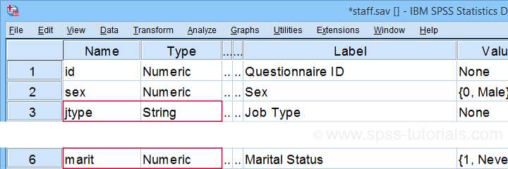
We encourage you to download and open this data file in SPSS and replicate the examples we'll present.
Prerequisites and Installation
Our tool requires SPSS version 24 or higher. Also, the SPSS Python 3 essentials must be installed (usually the case with recent SPSS versions).
Next, click SPSS_TUTORIALS_DUMMIFY.spe in order to download our tool. For installing it, navigate to
![]() as shown below.
as shown below.
In the dialog that opens, navigate to the downloaded .spe file and install it. SPSS will then confirm that the extension was successfully installed under
![]()
Example I - Numeric Categorical Variable
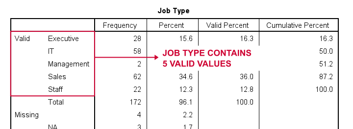
Let's now dummify Marital Status. Before doing so, we recommend you first inspect its basic frequency distribution as shown below.
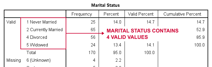
Importantly, note that Marital Status contains 4 valid (non missing) values. As we'll explain later on, we always need to exclude one category, known as the reference category. We'll therefore create 3 dummy variables to represent our 4 categories.
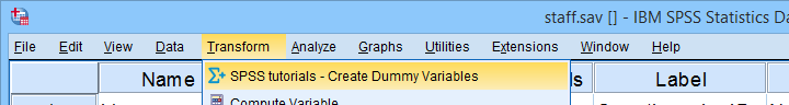
We'll do so by navigating to
![]() as shown below.
as shown below.
Let's now fill out the dialog that pops up.
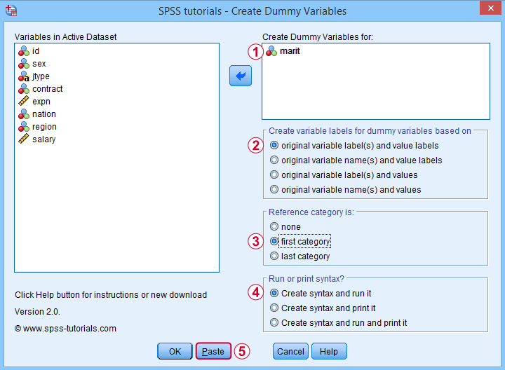
 We choose the first category (“Never Married”) as our reference category. Completing these results in the syntax below. Let's run it.
SPSS TUTORIALS DUMMIFY VARIABLES=marit
/OPTIONS NEWLABELS=LABLAB REFCAT=FIRST ACTION=RUN.
Result
Our tool has now created 3 dummy variables in the active dataset. Let's compare them to the value labels of our original variable, Marital Status.
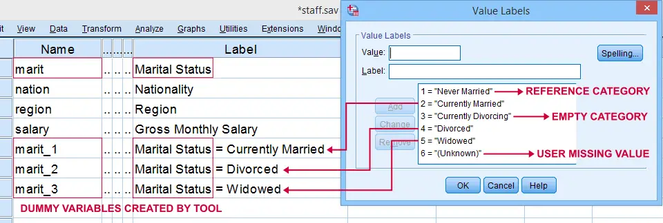
First note that the variable names for our dummy variables are the original variable name plus an integer suffix. These suffixes don't usually correspond to the categories they represent.
Instead, these categories are found in the variable labels for our dummy variables. In this example, they are based on the variable and value labels in Marital Status.
Next, note that some categories were skipped for the following reasons:
- no dummy variable was created for “Never Married” because we chose it as our reference category;
- no dummy variable was created for “Currently Divorcing” because it doesn't actually occur in our dataset;
- no dummy variable was created for “(Unknown)” because it is a user missing value.
Now the big question is:
are these results correct?
An easy way to confirm that they are indeed correct is actually running a dummy variable regression. We'll then run the exact same analysis with a basic ANOVA.
For example, let's try and predict Salary from Marital Status via both methods by running the syntax below.
regression
/dependent salary
/method enter marit_1 to marit_3.
*Compare mean salaries by marital status via ANOVA.
means salary by marit
/statistics anova.
First note that the regression r-square of 0.089 is identical to the eta squared of 0.089 in our ANOVA results. This makes sense because they both indicate the proportion of variance in Salary accounted for by Marital Status.
Also, our ANOVA comes up with a significance level of p = 0.002 just as our regression analysis does. We could even replicate the regression B-coefficients and their confidence intervals via ANOVA (we'll do so in a later tutorial). But for now, let's just conclude that the results are correct.
Example II - Categorical String Variable
Let's now dummify Job Type, a string variable. Again, we'll start off by inspecting its frequencies and we'll probably want to specify some missing values. As discussed in SPSS - Missing Values for String Variables, doing so is cumbersome but the syntax below does the job.
frequencies jtype.
*Change '(Unknown)' into 'NA'.
recode jtype ( '(Unknown)' = 'NA').
*Set empty string value and 'NA' as user missing values.
missing values jtype ('','NA').
*Reinspect basic frequency table.
frequencies jtype.
Result
Again, we'll first navigate to
![]() and we'll fill in the dialog as shown below.
and we'll fill in the dialog as shown below.
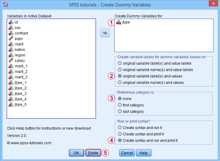
 For string variables, the values themselves usually describe their categories. We therefore throw values (instead of value labels) into the variable labels for our dummy variables.
If we neither want the first nor the last category as reference, we'll select “none”. In this case, we must manually exclude one of these dummy variables from the regression analysis that follows.
 Besides creating dummy variables, we may also want to inspect the syntax that's created and run by the tool. We may also copy, paste, edit and run it from a syntax window instead of having our tool do that for us.
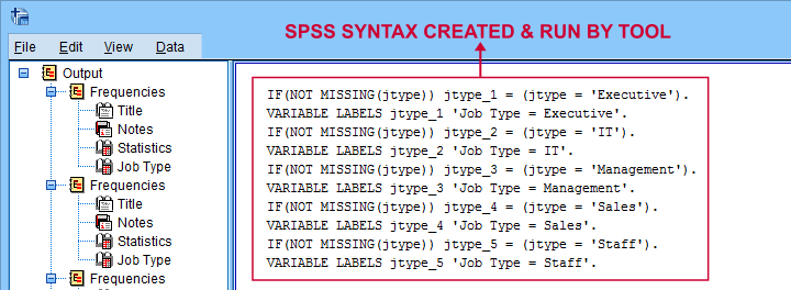
Completing these steps result in the syntax below.
SPSS TUTORIALS DUMMIFY VARIABLES=jtype
/OPTIONS NEWLABELS=LABVAL REFCAT=NONE ACTION=BOTH.
Result
Besides creating 5 dummy variables, our tool also prints the syntax that was used in the output window as shown below.
Finally, if you didn't choose any reference category, you must exclude one of the dummy variables from your regression analysis. The syntax below shows what happens if you don't.
regression
/dependent salary
/method enter jtype_1 jtype_2 jtype_3 jtype_4 jtype_5.
*Compare salaries by Job Type right way: reference category = 4 (sales).
regression
/dependent salary
/method enter jtype_1 jtype_2 jtype_3 jtype_5.
The first example is a textbook illustration of perfect multicollinearity: the score on some predictor can be perfectly predicted from some other predictor(s). This makes sense: a respondent scoring 0 on the first 4 dummies must score 1 on the last (and reversely).
In this situation, B-coefficients can't be estimated. Therefore, SPSS excludes a predictor from the analysis as shown below.
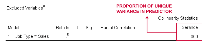
Note that tolerance is the proportion of variance in a predictor that can not be accounted for by other predictors in the model. A tolerance of 0.000 thus means that some predictor can be 100% -or perfectly- predicted from the other predictors.
Thanks for reading!
SPSS Scatterplots & Fit Lines Tool
Contents
- Example Data File
- Prerequisites and Installation
- Example I - Create All Unique Scatterplots
- Example II - Linearity Checks for Predictors
Visualizing your data is the single best thing you can do with it. Doing so may take little effort: a single line FREQUENCIES command in SPSS can create many histograms or bar charts in one go.
Sadly, the situation for scatterplots is different: each of them requires a separate command. We therefore built a tool for creating one, many or all scatterplots among a set of variables, optionally with (non)linear fit lines and regression tables.
Example Data File
We'll use health-costs.sav (partly shown below) throughout this tutorial.
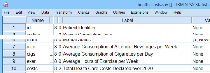
We encourage you to download and open this file and replicate the examples we'll present in a minute.
Prerequisites and Installation
Our tool requires SPSS version 24 or higher. Also, the SPSS Python 3 essentials must be installed (usually the case with recent SPSS versions).
Clicking SPSS_TUTORIALS_SCATTERS.spe downloads our scatterplots tool. You can install it through
![]() as shown below.
as shown below.
In the dialog that opens, navigate to the downloaded .spe file and install it. SPSS will then confirm that the extension was successfully installed under
![]()
Example I - Create All Unique Scatterplots
Let's now inspect all unique scatterplots among health costs, alcohol and cigarette consumption and exercise. We'll navigate to
![]() and fill out the dialog as shown below.
and fill out the dialog as shown below.
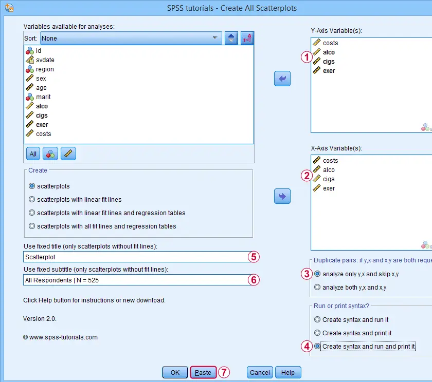
 We enter all relevant variables as y-axis variables. We recommend you always first enter the dependent variable (if any).
We enter these same variables as x-axis variables.
This combination of y-axis and x-axis variables results in duplicate chart. For instance, costs by alco is similar alco by costs transposed. Such duplicates are skipped if “analyze only y,x and skip x,y” is selected.
Besides creating scatterplots, we'll also take a quick look at the SPSS syntax that's generated.
 If no title is entered, our tool applies automatic titles. For this example, the automatic titles were rather lengthy. We therefore override them with a fixed title (“Scatterplot”) for all charts. The only way to have no titles at all is suppressing them with a chart template.
 Clicking results in the syntax below. Let's run it.
SPSS Scatterplots Tool - Syntax I
SPSS TUTORIALS SCATTERS YVARS=costs alco cigs exer XVARS=costs alco cigs exer
/OPTIONS ANALYSIS=SCATTERS ACTION=BOTH TITLE="Scatterplot" SUBTITLE="All Respondents | N = 525".
Results
First off, note that the GRAPH commands that were run by our tool have also been printed in the output window (shown below). You could copy, paste, edit and run these on any SPSS installation, even if it doesn't have our tool installed.
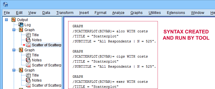
Beneath this syntax, we find all 6 unique scatterplots. Most of them show substantive correlations and all of them look plausible. However, do note that some plots -especially the first one- hint at some curvilinearity. We'll thoroughly investigate this in our second example.

In any case, we feel that a quick look at such scatterplots should always precede an SPSS correlation analysis.
Example II - Linearity Checks for Predictors
I'd now like to run a multiple regression analysis for predicting health costs from several predictors. But before doing so,
let's see if each predictor relates linearly
to our dependent variable. Again, we navigate to
![]() and fill out the dialog as shown below.
and fill out the dialog as shown below.
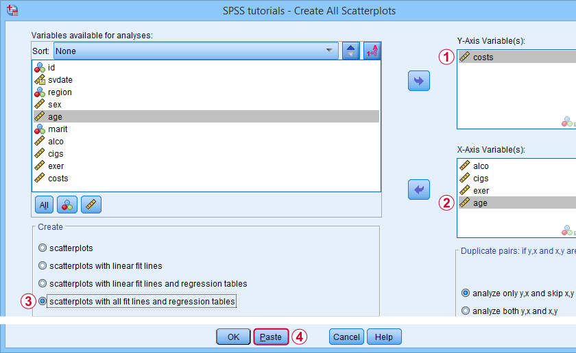
Our dependent variable is our y-axis variable.
All independent variables are x-axis variables.
We'll create scatterplots with all fit lines and regression tables.
We'll run the syntax below after clicking the button.
SPSS Scatterplots Tool - Syntax II
SPSS TUTORIALS SCATTERS YVARS=costs XVARS=alco cigs exer age
/OPTIONS ANALYSIS=FITALLTABLES ACTION=RUN.
Note that running this syntax triggers some warnings about zero values in some variables. These can safely be ignored for these examples.
Results
In our first scatterplot with regression lines, some curves deviate substantially from linearity as shown below.
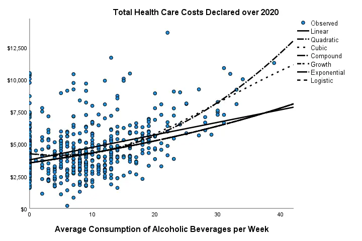
Sadly, this chart's legend doesn't quite help to identify which curve visualizes which transformation function. So let's look at the regression table shown below.
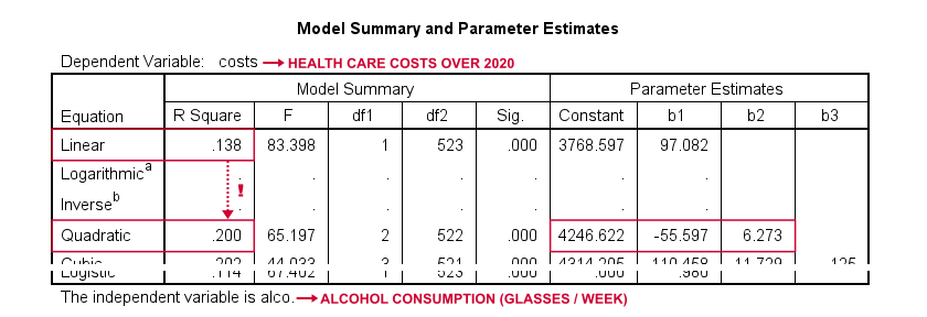
Very interestingly, r-square skyrockets from 0.138 to 0.200 when we add the squared predictor to our model. The b-coefficients tell us that the regression equation for this model is Costs’ = 4,246.22 - 55.597 * alco + 6.273 * alco2 Unfortunately, this table doesn't include significance levels or confidence intervals for these b-coefficients. However, these are easily obtained from a regression analysis after adding the squared predictor to our data. The syntax below does just that.
compute alco2 = alco**2.
*Multiple regression for costs on squared and non squared alcohol consumption.
regression
/statistics r coeff ci(95)
/dependent costs
/method enter alco alco2.
Result
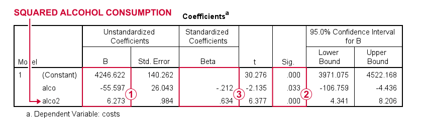
First note that we replicated the exact b-coefficients we saw earlier.
Surprisingly, our squared predictor is more statistically significant than its original, non squared counterpart.
The beta coefficients suggest that the relative strength of the squared predictor is roughly 3 times that of the original predictor.
In short, these results suggest substantial non linearity for at least one predictor. Interestingly, this is not detected by using the standard linearity check: inspecting a scatterplot of standardized residuals versus predicted values after running multiple regression.
But anyway, I just wanted to share the tool I built for these analyses and illustrate it with some typical examples. Hope you found it helpful!
If you've any feedback, we always appreciate if you throw us a comment below.
Thanks for reading!
SPSS – Recode with Value Labels Tool
This tutorial presents a simple tool for recoding values along with their value labels into different values.
- Prerequisites & Download
- Checking Results & Creating New Variables
- Example I - Reverse Code Variables
- Example II - Correct Order after AUTORECODE
- Example III - Convert 1-2 into 0-1 Coding
- Example IV - Correct Coding Errors with Native Syntax
Example Data
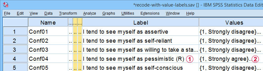
We'll use recode-with-value-labels.sav -partly shown below- for all examples.
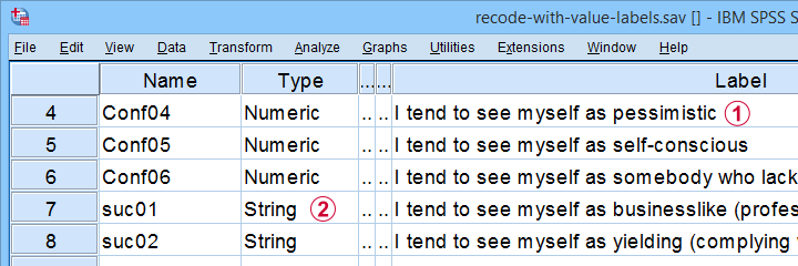
These data contain several common problems:
Some variables must be reverse coded because they measure the opposite of the other variables within some scale.
Some ordinal variables are coded as string variables.
The tool presented in this tutorial is the fastest option to fix these and several other common issues.
Prerequisites & Installation
Our recoding tool requires SPSS version 24+ with the SPSS Python 3 essentials properly installed -usually the case with recent SPSS versions.
Next, download our tool from SPSS_TUTORIALS_RECODE_WITH_VALUE_LABELS.spe. You can install it by dragging & dropping it into a data editor window. Alternatively, navigate to
![]() as shown below.
as shown below.
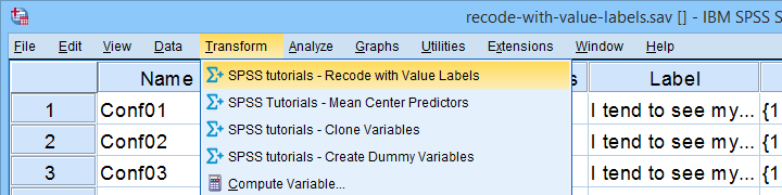
In the dialog that opens, navigate to the downloaded .spe file and select it. SPSS now throws a message that “The extension was successfully installed under Transform - SPSS tutorials - Recode with Value Labels”. You'll now find our tool under
![]() as shown below.
as shown below.
Checking Results & Creating New Variables
If you use our tool, you may want to verify that all result are correct. A basic way to do so is to compare some frequency distributions before and after recoding your variables. These will be identical (except for their order) if you show only value labels in your output.
Our tool modifies existing variables instead of creating new ones. If that's not to your liking, combine it with our SPSS Clone Variables Tool (shown below).
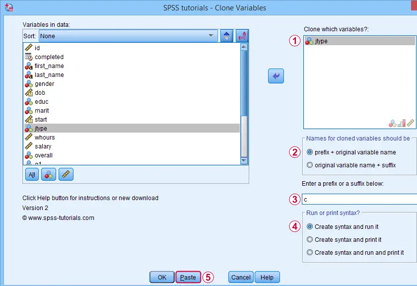
A very solid strategy is now to
- clone all variables you'd like to recode;
- recode the original (rather than the cloned) variables with our recoding tool;
- compare the recoded variables with their cloned counterparts with CROSSTABS;
- optionally: remove the cloned variables from your data when you're done.
Ok, so let's now see how our recoding tool solves some common data problems.
Example I - Reverse Code Variables
Conf01 to Conf06 are intended to measure self confidence. However, Conf04 and Conf06 indicate a lack of self confidence and correlate negatively with the other confidence items.
This issue is solved by reverse coding these items. After installing our tool, let's first navigate to
![]() Next, we'll fill out the dialogs as shown below.
Next, we'll fill out the dialogs as shown below.
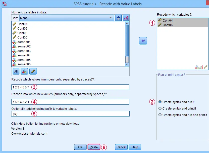
Excluding the user missing value of 8 (No answer) leaves this value and its value label unaltered.
Completing these steps results in the syntax below. Let's run it.
SPSS TUTORIALS RECODE_WITH_VALUE_LABELS VARIABLES=Conf04 Conf06 OLDVALUES=1 2 3 4 5 6 7 NEWVALUES=7
6 5 4 3 2 1
/OPTIONS LABELSUFFIX=" (R)" ACTION=RUN.
Result
Note that (R) is appended to the variable labels of our reverse coded variables;
The values and value labels have been reversed as well.
Our reverse coded items now correlate positively with all other confidence items as required for computing Cronbach’s alpha or a mean or sum score over this scale.
Example II - Correct Order after AUTORECODE
Another common issue are ordinal string variables in SPSS such as suc01 to suc06 which measure self-perceived successfulness. First off, let's convert them to labeled numeric variables by navigating to
![]() Next, we'll create an AUTORECODE command for a single variable as shown below.
Next, we'll create an AUTORECODE command for a single variable as shown below.
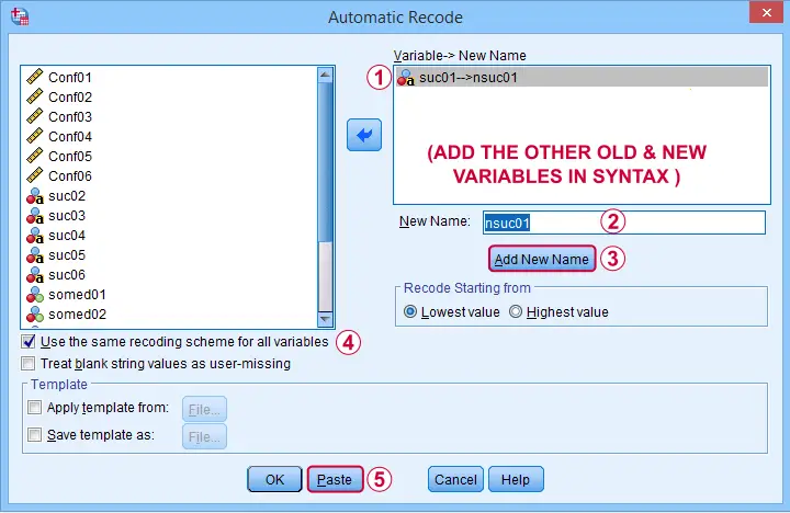
We can now easily add the remaining 5 variables to the resulting SPSS syntax as shown below. Let's run it.
AUTORECODE VARIABLES=suc01 to suc06 /* ADD ALL OLD VARIABLES HERE */
/INTO nsuc01 to nsuc06 /* ADD ALL NEW VARIABLES HERE */
/GROUP
/PRINT.
This syntax converts our string variables into numeric ones but the order of the answer categories is not as desired. For correcting this, we first copy-paste our new, numeric values into Notepad++ or Excel. This makes it easy to move them into the desired order as shown below.
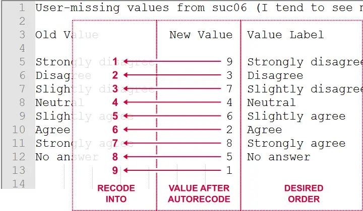
Doing so makes clear that we need to
- convert 9 into 1,
- convert 3 into 2,
- convert 7 into 3,
- and so on...
The figure below shows how to do so with our recoding tool.
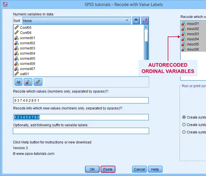
This results in the syntax below, which sets the correct order for our autorecoded numeric variables.
SPSS TUTORIALS RECODE_WITH_VALUE_LABELS VARIABLES=nsuc01 nsuc02 nsuc03 nsuc04 nsuc05 nsuc06
OLDVALUES=9 3 7 4 6 2 8 5 1 NEWVALUES=1 2 3 4 5 6 7 8 9
/OPTIONS ACTION=RUN.
Example III - Convert 1-2 into 0-1 Coding
In SPSS, we preferably use a 0-1 coding for dichotomous variables. Some reasons are that
- this facilitates interpreting b-coefficients for dummy variables in multiple regression;
- means for 0-1 coded variables correspond to proportions of “yes” answers which are easily interpretable.
The syntax below is easily created with our recoding tool and converts the 1-2 coding for all dichotomous variables in our data file into a 0-1 coding.
SPSS TUTORIALS RECODE_WITH_VALUE_LABELS VARIABLES=somed01 somed02 somed03 somed04 somed05 somed06
somed07 OLDVALUES=2 NEWVALUES=0
/OPTIONS ACTION=RUN.
Example IV - Correct Coding Errors with Native Syntax
If we take a close look at our final variable, sat01, we see that it is coded 21 through 27. Depending on how we analyze it, we may want to convert it into a standard 7-point Likert scale. The screenshot below shows how it's done.
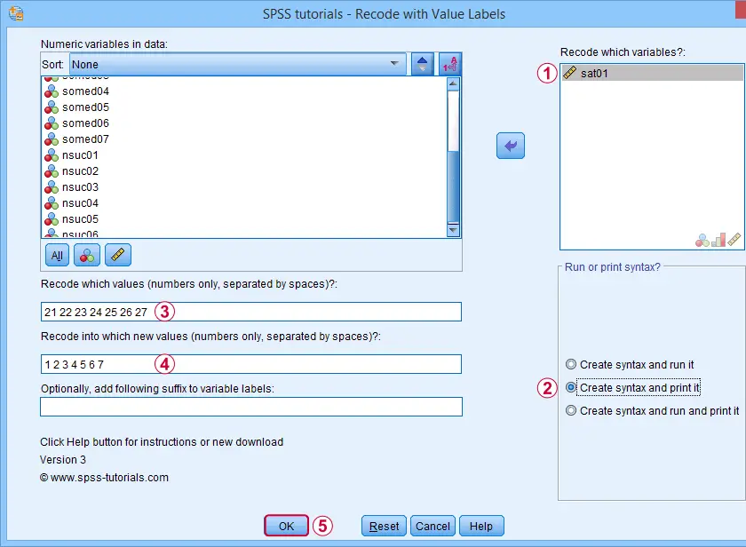
Note that we select “Create syntax and print it” for creating native syntax.
Result
As shown below, selecting the print option results in native SPSS syntax in your output window.
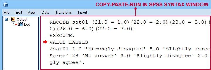
The syntax we thus copy-pasted from our output window is:
RECODE sat01 (21.0 = 1.0)(22.0 = 2.0)(23.0 = 3.0)(24.0 = 4.0)(25.0 = 5.0)(26.0 = 6.0)(27.0 = 7.0).
EXECUTE.
VALUE LABELS
/sat01 1.0 'Strongly disagree' 2.0 'Disagree' 3.0 'Slightly disagree' 4.0 'Neutral' 5.0 'Slightly agree' 6.0 'Agree' 7.0 'Strongly agree'.
Note that it consists of 3 very basic commands:
- RECODE adjusts the values themselves;
- EXECUTE can usually be removed from the syntax but it ensures that our RECODE is executed immediately;
- VALUE LABELS adjusts our value labels after our RECODE.
So why should you consider using the print option? Well, the default syntax created by our tool only runs on SPSS installations with the tool installed. So if a client or colleague needs to replicate your work,
using native syntax ensures that everything will run
on any SPSS installation.
Right, so that should do. I hope you'll find my tool helpful -I've been using it on tons of project myself. If you've any questions or remarks, just throw me a comment below, ok?
Thanks for reading!
SPSS Clone Variables Tool
Some SPSS commands such as RECODE and ALTER TYPE can make irreversible changes to variables. Before using these, I like to clone the variables that I'm about to edit. This allows me to compare the edited to the original versions.
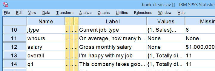
This tutorial presents a super easy tool for making exact clones of variables in SPSS. We'll use bank-clean.sav (partly shown below) for all examples.
Prerequisites & Installation
Installing this tool requires
- SPSS version 24 or higher with
- the SPSS Python 3 essentials installed.
Recent SPSS versions usually meet these requirements.
Download our tool from SPSS_TUTORIALS_CLONE_VARIABLES.spe. You can install it from
![]() as shown below.
as shown below.
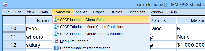
After completing these steps, you'll find SPSS tutorials - Clone Variables under Transform.
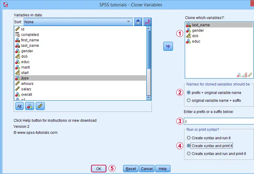
Clone Variables Example I
Let's first clone jtype -short for job type- as illustrated below.
Completing these steps results in the SPSS syntax below. Let's run it.
SPSS_TUTORIALS_CLONE_VARIABLES VARIABLES=jtype
/OPTIONS FIX="c" FIXTYPE=PREFIX ACTION=RUN.
Result
Note that SPSS has now added a new variable to our data: cjtype as shown below.
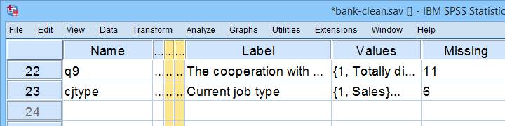
Except for its name, cjtype is an exact clone of jtype: it has the same
- variable type and format;
- value labels;
- user missing values;
- and so on...
There's one minor issue with our first example: the syntax we just pasted only runs on SPSS installations with our tool installed.
The solution for this is to have the tool print native syntax instead: this syntax is typically (much) longer but it does run on any SPSS installation. Our second examples illustrates how to do just that.
Clone Variables Example II
Let's create native syntax for cloning a couple of different variables, including a string variable and a date variable.
 This option has our tool print native syntax into our output window.
 Because we chose to print (rather than run) syntax, this is one of the rare occasions at which we click Ok instead of Paste.
Result
Note that we now have native syntax for cloning several variables in our output window.
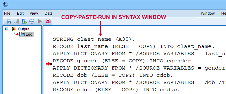
For actually running this syntax, we can simply copy-paste-run it in a syntax window.The entire syntax is shown below.
STRING clast_name (A30).
RECODE last_name (ELSE = COPY) INTO clast_name.
APPLY DICTIONARY FROM * /SOURCE VARIABLES = last_name /TARGET VARIABLES = clast_name.
RECODE gender (ELSE = COPY) INTO cgender.
APPLY DICTIONARY FROM * /SOURCE VARIABLES = gender /TARGET VARIABLES = cgender.
RECODE dob (ELSE = COPY) INTO cdob.
APPLY DICTIONARY FROM * /SOURCE VARIABLES = dob /TARGET VARIABLES = cdob.
RECODE educ (ELSE = COPY) INTO ceduc.
APPLY DICTIONARY FROM * /SOURCE VARIABLES = educ /TARGET VARIABLES = ceduc.
If our tool creates very long syntax, you could copy it into a separate file and run it from an INSERT command.
Right, I guess that should cover this simple but handy little tool. Hope you'll give it a try and hope you'll find it helpful. If you've any remarks, feel free to throw me a quick comment below.
Thanks for reading!
SPSS VARSTOCASES With Labels Tool

Running VARSTOCASES is often necessary for generating nice charts in SPSS. One of the many examples is a stacked bar chart for comparing multiple variables. Sadly, we lose our variable labels when running VARSTOCASES and we really do need those.
The solution is a simple tool that generates our VARSTOCASES for us and applies the variable labels of the input variables as value labels to the newly created index variable.
SPSS VARSTOCASES Problem - Example
Before proposing our solution, let's first take a look at the problem. We'll use course_evaluation.sav, part of which is shown below.
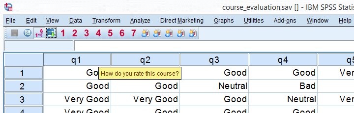
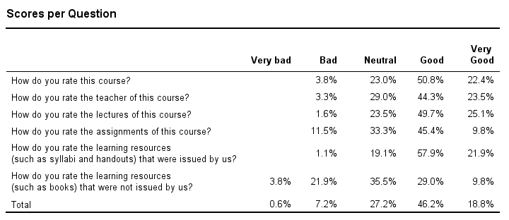
Now let's say we'd like to create the overview table shown below, perhaps followed up by a nice chart. The way to go here is VARSTOCASES as we'll demonstrate in a minute.
Desired End Result
Quick Data Check before VARSTOCASES
Whenever running VARSTOCASES, we always need to make sure our input variables have consistent value labels as explained in VARSTOCASES - wrong results. We'll check that by running the syntax below.
Inspecting Consistency of Value Labels Syntax
set tnumbers both.
*2. Check if value labels are consistent over variables.
frequencies q1 to q6.
*Result: consistent labels, good to go.
Right, we now run a basic VARSTOCASES command followed by CROSSTABS for comparing the scores on our 6 input variables in a single table.
Creating an Overview Table Syntax
varstocases/make q from q1 to q6/index question (q).
*2. Show only labels in output for reporting.
set tnumbers labels tvars labels.
*3. Create table.
crosstabs question by q/cells row.
Result
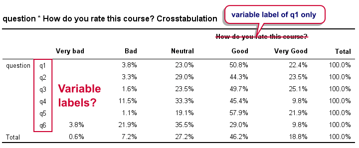
Right. Now, the numbers in this table are correct but we find it very annoying that we lost the variable labels for q2 to q6 in the process. By default, the variable label for q1 is -incorrectly- applied to our newly created variable that now holds the values of q1 to q6. It's precisely these two problems that our tool takes care of.
VARSTOCASES with Labels Tool - How to Use It?
- This tool requires SPSS version 17 or higher with the SPSS Python Essentials properly installed.
- Download and install the VARSTOCASES with labels tool. Note that this is an SPSS custom dialog.
- Navigate to
 .
. - Enter the input variables. Note that you can use the TO and ALL keywords for doing so.
- and run the syntax.
- directs your web browser to the tutorial you're currently reading.
VARSTOCASES with Labels Tool - Just Do It
If you already ran VARSTOCASES on course_evaluation.sav, then you'll need to reopen the original data. After installing the tool, you'll find it under in the menu. Fill it out as shown below.
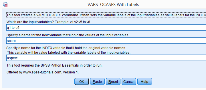
Clicking results in the syntax below.
VARSTOCASES Syntax Generated by Tool
dataset close all.
new file.
get file 'course_evaluation.sav'.
*2. SPSS Python syntax pasted from tool.
begin program.
varSpec = 'q1 to q6'
import spssaux,spss
vallabcmd = 'value labels aspect'
sDict = spssaux.VariableDict(caseless = True)
varList = sDict.expand(varSpec)
for var in varList:
vallabcmd += "\n'%s' '%s'"%(var.lower(),sDict[var].VariableLabel)
spss.Submit('''
varstocases/make score '' from q1 to q6/index aspect(score).
compute aspect = lower(aspect).
''')
spss.Submit(vallabcmd + '.')
end program.
Generating a Nice Overview Table
After running the previous example, we're good to go. We'll now create a nice overview table of q1 to q6 by running the syntax below.
variable labels q "Answer Category".
*2. Generate table.
crosstabs question by q/cells row.
Result
Final Notes
Our final table can also be created with CTABLES but not all SPSS users have a license for it. Alternatively, TABLES can do the trick but it's available only from (rather challenging) syntax which is no longer documented.
In our daily work, we routinely use this tool for creating charts rather than tables. One example, the stacked bar chart will be discussed in next week’s tutorial.
SPSS – Confidence Intervals for Correlations Tool
Summary
What's the easiest way to obtain confidence intervals for Pearson correlations? Sadly, we couldn't find these often requested statistics anywhere in SPSS. The best we encountered on the web were some ancient macros that aren't exactly user friendly.
This tutorial therefore proposes a freely downloadable, menu based tool for computing one or many confidence intervals for Pearson correlations.
How to Use the Tool?
- This tool requires SPSS version 17 or higher with the SPSS Python Essentials properly installed and running. If you don't have that available, you can use this plain syntax version instead of the actual tool.
- Download and install the Confidence Intervals for Correlations Tool. Note that this is an SPSS custom dialog.
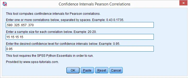
- Navigate to .
- Fill in one or more correlations. Use your locale's decimal separator. That's usually a dot but some European languages use a comma. If you're not sure: the dialog’s default confidence level uses the separator appropriate for your locale.
- Fill in the corresponding sample sizes. The number of sample sizes should be equal to the number of correlations you enter.
- Fill in a single confidence level for all correlations. Click .
- Note that clicking directs you to the online tutorial you're currently reading.
Output
Running the tool results in SPSS creating a new dataset as shown below.
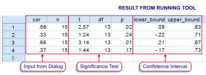
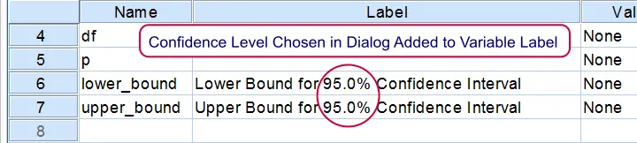
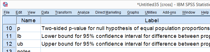
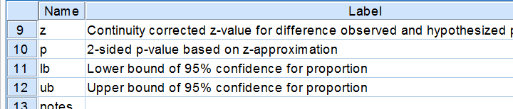
If you're unsure which confidence level you requested, switch from data view to variable view. The confidence level is added to the variable labels of the lower and upper bounds as shown below.
Theory
The sampling distribution for a correlation approaches a normal distribution only as the sample size becomes very large. However, the result of the following non linear transformation reasonably approximates a normal distribution when n > 10:
$$E(Z_F) \approx \frac{1}{2} \ln \frac{1 + \rho}{1 - \rho} + \frac{\rho}{2(n - 1)}$$
This formula is known as Fisher’s z-transformation. After applying it, the standard normal distribution is used for computing confidence intervals for the transformed correlations.
Finally, the upper and lower bounds for the transformed correlations are converted back to “normal correlations” by reversing the aforementioned formula by means of a Newton-Raphson approximation.
We'd like to thank our colleague Reinoud Hamming from ![]() TNS NIPO for his kind assistance with the formulas.
TNS NIPO for his kind assistance with the formulas.
SPSS Z-Test for 2 Independent Proportions Tool
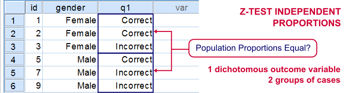
If you'd like to know if 2 groups of people score similarly on 1 dichotomous variable, you'll compare 2 independent proportions. There's two basic ways to do so:
- the chi-square independence test and;
- the z-test for 2 independent proportions.
These tests yield identical p-values but the z-test approach allows you to compute a confidence interval for the difference between the proportions. Unfortunately, this very basic test is painfully absent from SPSS. We'll therefore present a freely downloadable tool for it in the remainder of this tutorial.
Installation
- This tool requires SPSS version 18 or higher with the SPSS Python Essentials properly installed and tested.
- Download the Confidence Intervals Independent Proportions tool.
- For SPSS versions 18 through 22, select . For SPSS 24, select .
Navigate to the confidence intervals extension (its file name ends in “.spe”, short for SPSS Extension) and install it. - Although you'll get a popup that the extension was successfully installed, it'll only work after you close and reopen SPSS entirely (unless you're on version 24).
- You'll now find the tool under .
Operations
- Make sure the grouping variable has exactly two valid values. If this doesn't hold, the tool will throw a fatal error pointing out the problem.
- The grouping variable may be a numeric variable or a string variable. If it's a string, keep in mind that empty string values are valid by default in SPSS but you can specify them as user missing values.
- The test variables must have exactly two valid values as well. Variables violating this requirement will be skipped when calculating results.
- The test variables may be any mixture of numeric and string variables.
- The p-values and confidence intervals are based on the normal distribution. This approximation is sufficiently accurate if p1*n1, (1-p1)*n1, p2*n2 and (1-p2)*n2 are all > 5, where p and n denote the two test proportions and their related sample sizes.1 If this does not hold, a warning will be added to the results.
- If any SPLIT FILE is in effect, the tool will switch if off, throw a warning that it did so and then proceed as usual.
- If a WEIGHT variable is in effect, results will be based on rounded frequencies. P-values may be biased if you're using non integer sampling weights but this holds for all p-values in SPSS except for those from the complex samples module.2,3,4
Example
Let's just try things out on test.sav, part of which is shown below. We'll test if men and women score differently on separate items.
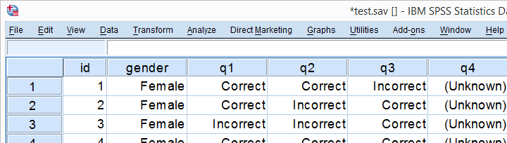
Data Inspection
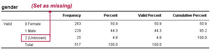
We'll first see if we need to specify any user missing values by running the syntax below.
set tnumbers both.
*See if all variables have exactly two valid values.
frequencies gender to passes.
*Set missing values as needed. The tiny mistake here of omitting q5 is deliberate.
missing values gender to q4 (2).
*Show only value labels in output.
set tnumbers labels.
Result
Crosstabs
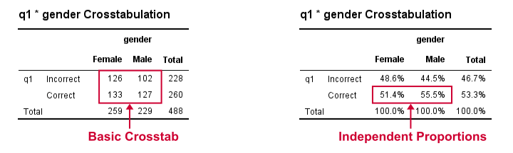
We'll now run some super basic CROSSTABS. We'll normally skip this step but for now they'll help us understand the results from our tool that we'll see in a minute.
crosstabs q1 by gender.
*Independent proportions.
crosstabs q1 by gender/cells column.
Result
Computing our Confidence Intervals
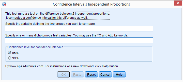
We'll select ![]() and fill out the main dialog as below.
and fill out the main dialog as below.
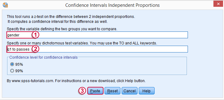
Note that TO may be used for a range of variable names.
 Clicking results in the syntax below.
CONFIDENCE_INTERVALS_INDEPENDENT_PROPORTIONS GROUP = 'gender' VARIABLES = 'q1 to passes' LEVEL = 95.
Results
Upon running our syntax, a new dataset will pop up holding both crosstabs we saw earlier for each test variable. Note that most variables have variable labels explaining their precise meaning. You can see them in variable view or hover over a variable’s name in data view as shown in the screenshot below.
The crosstab with frequencies holds the input data for our calculations. The crosstab with percentages (screenshot below) holds our test proportions. Each test variable results in 2 rows, one for each value. You'll typically need just one but the setup chosen here makes the interface efficient and flexible.
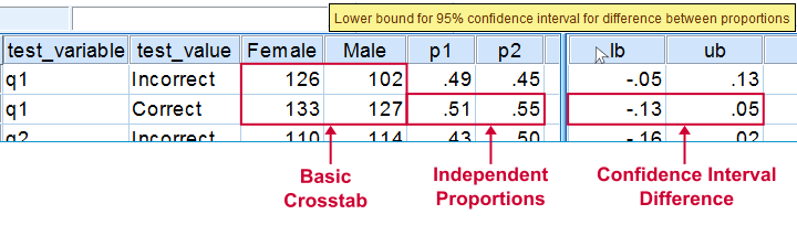
Further right we find our z-test. Its p-value indicates the probability of finding the observed difference between our independent proportions if the population difference is zero. The p-values are identical of those yielded by Pearson’s chi-square in CROSSTABS.
We then encounter our confidence intervals. Last but not least, we may or may not have some notes (in this case we do).
That's it. I hope you'll find this tool useful. Please let me know by leaving a comment. Thank you!
References
- Van den Brink, W.P. & Koele, P. (2002). Statistiek, deel 3 [Statistics, part 3]. Amsterdam: Boom.
- Fowler, F.J. (2009). Survey Research Methods. Thousand Oaks, CA: SAGE.
- De Leeuw, E.D., Hox, J.J. and Dillman, D.A. (2008). International Handbook of Survey Methodology. New York: Lawrence Erlbaum Associates.
- Kish, L. Weighting for Unequal Pi. Journal of Official Statistics, 8, 183-200.
Z-Test and Confidence Interval Proportion Tool
There's two basic tests for testing a single proportion:
- the binomial test and
- the z-test for a single proportion.
For larger samples, these tests result in roughly similar p-values. However, the binomial test only comes up with a 1-tailed p-value unless the hypothesized proportion = 0.5. Moreover, it can't compute a confidence interval for your proportion.
The z-test does not have these 2 limitations and is among the more widely used statistical tests. Very oddly, however, it's absent from SPSS. Plenty of reasons for us to present this very simple tool in the remainder of this tutorial.
Installation
- This tool requires SPSS version 18 or higher with the SPSS Python Essentials properly installed and tested.
- Download the Confidence Interval Proportion tool.
- For SPSS versions 18 through 22, select . For SPSS 24, select .
Navigate to the confidence intervals extension (its file name ends in “.spe”, short for SPSS Extension) and install it. - Although you'll get a popup that the extension was successfully installed, it'll only work after you close and reopen SPSS entirely (unless you're on version 24).
- You'll now find the tool under .
Operations
- The test variables must have exactly two valid values. Variables violating this requirement will be skipped when calculating results.
- The test variables may be any mixture of numeric and string variables.
- The p-values and confidence intervals are based on the central limit theorem. This approximation is sufficiently accurate if p0*n and (1-p0)*n >5 where p0 denotes the population proportion under H0 and n is its related sample size.1 If this does not hold for one or more variables, a note will be added to the results.
- If any SPLIT FILE is in effect, the tool will switch if off, throw a warning that it did so and then proceed as usual.
- If a WEIGHT variable is in effect, results will be based on rounded frequencies. P-values may be biased if you're using non integer sampling weights but this holds for all p-values in SPSS except for those from the complex samples module.2,3,4
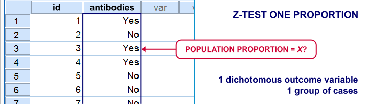
Example
We'll now test our tool on test.sav, part of which is shown below. Our null hypothesis is that the population proportions of all dichotomous variables = 0.5.
Data Inspection
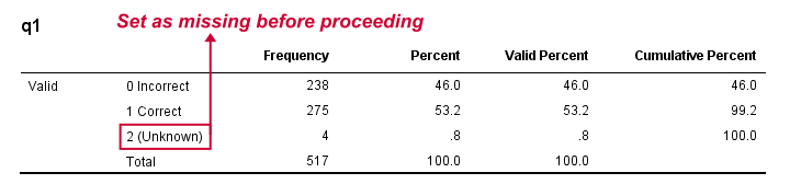
We'll run a quick data check with FREQUENCIES to see if we need to specify any user missing values. This happens to be the case so we'll do just that.
set tnumbers both.
*Basic frequency tables.
frequencies q1 to passes.
*Set missing values.
missing values q1 to q4 (2).
*Show only value labels in output.
set tnumbers labels.
Result
Computing our Confidence Intervals
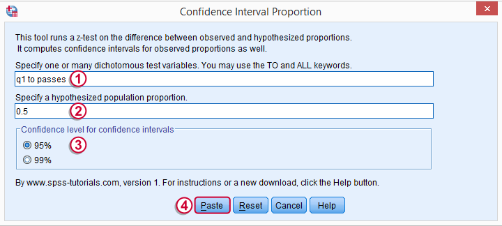
We'll go to ![]() and fill out the main dialog as below.
and fill out the main dialog as below.
 Note that TO may be used for a range of variable names.
Clicking results in the syntax below.
CONFIDENCE_INTERVAL_PROPORTION VARIABLES = 'q1 to passes' TESTPROP = 0.5 LEVEL = 95.
Results
Running our syntax results in a new dataset holding our results. Note that most variables have variable labels explaining their precise meaning. You can see them in variable view or hover over a variable’s name in data view as shown in the screenshot below.
We find back our (valid) frequencies in these results. Each test variable has in 2 rows, one for each value. You'll probably need just one of these rows but this configuration circumvents the need for specifying test values for each variable. We simply test both -whatever they may be.
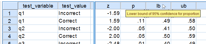
Further right we find our z-test. Its p-value indicates the probability of finding the observed sample proportions if its population counterpart is exactly equal to the test proportion. Note that a continuity correction has been used for computing the z-values and their associated p-values. Finally, the last variables in our results hold our confidence intervals and -possibly- some notes on the results.
Reporting Examples
Obviously, include your sample proportions and sample size in your report. Regarding the z-tests, we'll write something like “the proportion of people who answered q1 correctly did not differ from 0.5, as indicated by a z-test: z = 1.59, p = 0.11.”or “A z-test showed that more than 50% of our population answers q2 correctly, z = 2.0, p = 0.046.”
Thanks for reading, hope you'll like it!
References
- Van den Brink, W.P. & Koele, P. (2002). Statistiek, deel 3 [Statistics, part 3]. Amsterdam: Boom.
- Fowler, F.J. (2009). Survey Research Methods. Thousand Oaks, CA: SAGE.
- De Leeuw, E.D., Hox, J.J. and Dillman, D.A. (2008). International Handbook of Survey Methodology. New York: Lawrence Erlbaum Associates.
- Kish, L. Weighting for Unequal Pi. Journal of Official Statistics, 8, 183-200.