Cohen’s D – Effect Size for T-Test
Cohen’s D is the difference between 2 means
expressed in standard deviations.
- Cohen’s D - Formulas
- Cohen’s D and Power
- Cohen’s D & Point-Biserial Correlation
- Cohen’s D - Interpretation
- Cohen’s D for SPSS Users
Why Do We Need Cohen’s D?
Children from married and divorced parents completed some psychological tests: anxiety, depression and others. For comparing these 2 groups of children, their mean scores were compared using independent samples t-tests. The results are shown below.
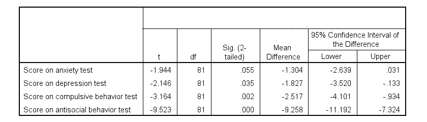
Some basic conclusions are that
- all mean differences are negative. So the second group -children from divorced parents- have higher means on all tests.
- Except for the anxiety test, all differences are statistically significant.
- The mean differences range from -1.3 points to -9.3 points.
However, what we really want to know is are these small, medium or large differences? This is hard to answer for 2 reasons:
- psychological test scores don't have any fixed unit of measurement such as meters, dollars or seconds.
- Statistical significance does not imply practical significance (or reversely). This is because p-values strongly depend on sample sizes.
A solution to both problems is using the standard deviation as a unit of measurement like we do when computing z-scores. And a mean difference expressed in standard deviations -Cohen’s D- is an interpretable effect size measure for t-tests.
Cohen’s D - Formulas
Cohen’s D is computed as
$$D = \frac{M_1 - M_2}{S_p}$$
where
- \(M_1\) and \(M_2\) denote the sample means for groups 1 and 2 and
- \(S_p\) denotes the pooled estimated population standard deviation.
But precisely what is the “pooled estimated population standard deviation”? Well, the independent-samples t-test assumes that the 2 groups we compare have the same population standard deviation. And we estimate it by “pooling” our 2 sample standard deviations with
$$S_p = \sqrt{\frac{(N_1 - 1) \cdot S_1^2 + (N_2 - 1) \cdot S_2^2}{N_1 + N_2 - 2}}$$
Fortunately, we rarely need this formula: SPSS, JASP and Excel readily compute a t-test with Cohen’s D for us.
Cohen’s D in JASP
Running the exact same t-tests in JASP and requesting “effect size” with confidence intervals results in the output shown below.
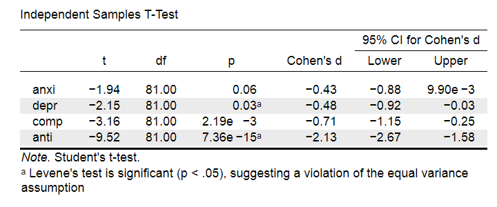
Note that Cohen’s D ranges from -0.43 through -2.13. Some minimal guidelines are that
- d = 0.20 indicates a small effect,
- d = 0.50 indicates a medium effect and
- d = 0.80 indicates a large effect.
And there we have it. Roughly speaking, the effects for
- the anxiety (d = -0.43) and depression tests (d = -0.48) are medium;
- the compulsive behavior test (d = -0.71) is fairly large;
- the antisocial behavior test (d = -2.13) is absolutely huge.
We'll go into the interpretation of Cohen’s D into much more detail later on. Let's first see how Cohen’s D relates to power and the point-biserial correlation, a different effect size measure for a t-test.
Cohen’s D and Power
Very interestingly, the power for a t-test can be computed directly from Cohen’s D. This requires specifying both sample sizes and α, usually 0.05. The illustration below -created with G*Power- shows how power increases with total sample size. It assumes that both samples are equally large.
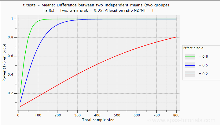
If we test at α = 0.05 and we want power (1 - β) = 0.8 then
- use 2 samples of n = 26 (total N = 52) if we expect d = 0.8 (large effect);
- use 2 samples of n = 64 (total N = 128) if we expect d = 0.5 (medium effect);
- use 2 samples of n = 394 (total N = 788) if we expect d = 0.2 (small effect);
Cohen’s D and Overlapping Distributions
The assumptions for an independent-samples t-test are
- independent observations;
- normality: the outcome variable must be normally distributed in each subpopulation;
- homogeneity: both subpopulations must have equal population standard deviations and -hence- variances.
If assumptions 2 and 3 are perfectly met, then Cohen’s D implies which percentage of the frequency distributions overlap. The example below shows how some male population overlaps with some 69% of some female population when Cohen’s D = 0.8, a large effect.
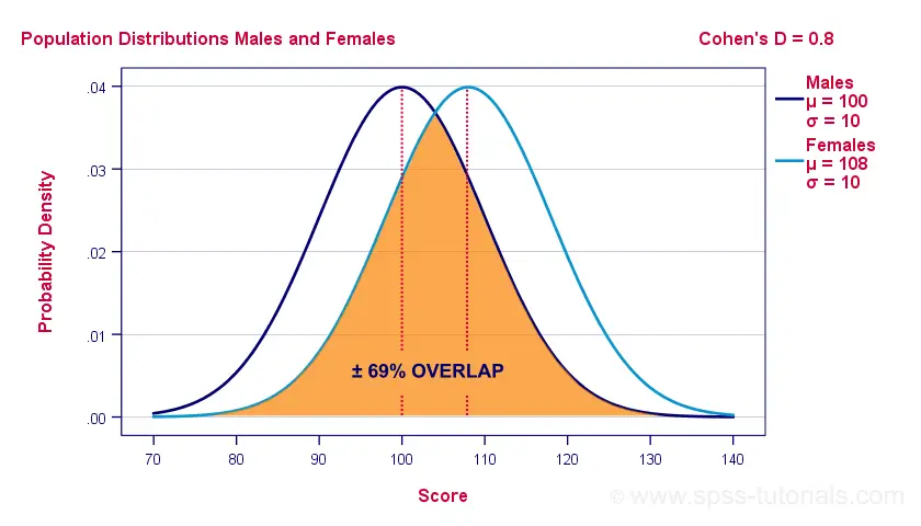
The percentage of overlap increases as Cohen’s D decreases. In this case, the distribution midpoints move towards each other. Some basic benchmarks are included in the interpretation table which we'll present in a minute.
Cohen’s D & Point-Biserial Correlation
An alternative effect size measure for the independent-samples t-test is \(R_{pb}\), the point-biserial correlation. This is simply a Pearson correlation between a quantitative and a dichotomous variable. It can be computed from Cohen’s D with
$$R_{pb} = \frac{D}{\sqrt{D^2 + 4}}$$
For our 3 benchmark values,
- Cohen’s d = 0.2 implies \(R_{pb}\) ± 0.100;
- Cohen’s d = 0.5 implies \(R_{pb}\) ± 0.243;
- Cohen’s d = 0.8 implies \(R_{pb}\) ± 0.371.
Alternatively, compute \(R_{pb}\) from the t-value and its degrees of freedom with
$$R_{pb} = \sqrt{\frac{t^2}{t^2 + df}}$$
Cohen’s D - Interpretation
The table below summarizes the rules of thumb regarding Cohen’s D that we discussed in the previous paragraphs.
| Cohen’s D | Interpretation | Rpb | % overlap | Recommended N |
|---|---|---|---|---|
| d = 0.2 | Small effect | ± 0.100 | ± 92% | 788 |
| d = 0.5 | Medium effect | ± 0.243 | ± 80% | 128 |
| d = 0.8 | Large effect | ± 0.371 | ± 69% | 52 |
Cohen’s D for SPSS Users
Cohen’s D is available in SPSS versions 27 and higher. It's obtained from
![]()
![]() as shown below.
as shown below.
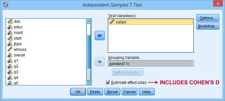
For more details on the output, please consult SPSS Independent Samples T-Test.
If you're using SPSS version 26 or lower, you can use Cohens-d.xlsx. This Excel sheet recomputes all output for one or many t-tests including Cohen’s D and its confidence interval from
- both sample sizes,
- both sample means and
- both sample standard deviations.
The input for our example data in divorced.sav and a tiny section of the resulting output is shown below.
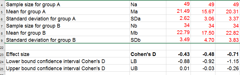
Note that the Excel tool doesn't require the raw data: a handful of descriptive statistics -possibly from a printed article- is sufficient.
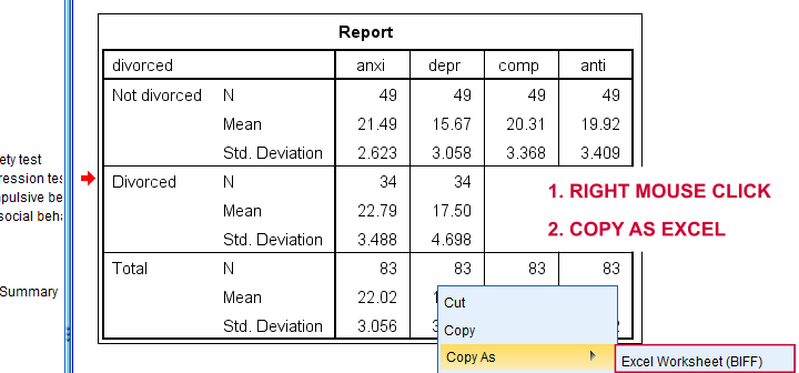
SPSS users can easily create the required input from a simple MEANS command if it includes at least 2 variables. An example is
means anxi to anti by divorced
/cells count mean stddev.
Copy-pasting the SPSS output table as Excel preserves the (hidden) decimals of the results. These can be made visible in Excel and reduce rounding inaccuracies.
Final Notes
I think Cohen’s D is useful but I still prefer R2, the squared (Pearson) correlation between the independent and dependent variable. Note that this is perfectly valid for dichotomous variables and also serves as the fundament for dummy variable regression.
The reason I prefer R2 is that it's in line with other effect size measures: the independent-samples t-test is a special case of ANOVA. And if we run a t-test as an ANOVA, η2 (eta squared) = R2 or the proportion of variance accounted for by the independent variable. This raises the question:
why should we use a different effect size measure
if we compare 2 instead of 3+ subpopulations?
I think we shouldn't.
This line of reasoning also argues against reporting 1-tailed significance for t-tests: if we run a t-test as an ANOVA, the p-value is always the 2-tailed significance for the corresponding t-test. So why should you report a different measure for comparing 2 instead of 3+ means?
But anyway, that'll do for today. If you've any feedback -positive or negative- please drop us a comment below. And last but not least:
thanks for reading!
One-Sample T-Test – Quick Tutorial & Example
A one-sample t-test evaluates if a population mean
is likely to be x: some hypothesized value.
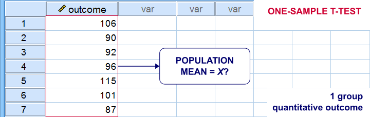
One-Sample T-Test Example
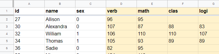
A school director thinks his students perform poorly due to low IQ scores. Now, most IQ tests have been calibrated to have a mean of 100 points in the general population. So the question is does the student population have a mean IQ score of 100? Now, our school has 1,114 students and the IQ tests are somewhat costly to administer. Our director therefore draws a simple random sample of N = 38 students and tests them on 4 IQ components:
- verb (Verbal Intelligence )
- math (Mathematical Ability )
- clas (Classification Skills )
- logi (Logical Reasoning Skills)
The raw data thus collected are in this Googlesheet, partly shown below. Note that a couple of scores are missing due to illness and unknown reasons.
Null Hypothesis
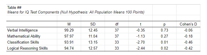
We'll try to demonstrate that our students have low IQ scores by rejecting the null hypothesis that the mean IQ score for the entire student population is 100 for each of the 4 IQ components measured. Our main challenge is that we only have data on a sample of 38 students from a population of N = 1,114. But let's first just look at some descriptive statistics for each component:
- N - sample size;
- M - sample mean and
- SD - sample standard deviation.
Descriptive Statistics
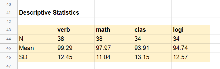
Our first basic conclusion is that our 38 students score lower than 100 points on all 4 IQ components. The differences for verb (99.29) and math (97.97) are small. Those for clas (93.91) and logi (94.74) seem somewhat more serious.
Now, our sample of 38 students may obviously come up with slightly different means than our population of N = 1,114. So
what can we (not) conclude regarding our population?
We'll try to generalize these sample results to our population with 2 different approaches:
- Statistical significance: how likely are these sample means if the population means are really all 100 points?
- Confidence intervals: given the sample results, what are likely ranges for the population means?
Both approaches require some assumptions so let's first look into those.
Assumptions
The assumptions required for our one-sample t-tests are
- independent observations and
- normality: the IQ scores must be normally distributed in the entire population.
Do our data meet these assumptions? First off,
1. our students didn't interact during their tests. Therefore, our observations are likely to be independent.
2. Normality is only needed for small sample sizes, say N < 25 or so. For the data at hand, normality is no issue. For smaller sample sizes, you could evaluate the normality assumption by
- inspecting if the histograms roughly follow normal curves,
- inspecting if both skewness and kurtosis are close to 0 and
- running a Shapiro-Wilk test or a Kolmogorov-Smirnov test.
However, the data at hand meet all assumptions so let's now look into the actual tests.
Formulas
If we'd draw many samples of students, such samples would come up with different means. We can compute the standard deviation of those means over hypothesized samples: the standard error of the mean or \(SE_{mean}\)
$$SE_{mean} = \frac{SD}{\sqrt{N}}$$
for our first IQ component, this results in
$$SE_{mean} = \frac{12.45}{\sqrt{38}} = 2.02$$
Our null hypothesis is that the population mean, \(\mu_0 = 100\). If this is true, then the average sample mean should also be 100. We now basically compute the z-score for our sample mean: the test statistic \(t\)
$$t = \frac{M - \mu_0}{SE_{mean}}$$
for our first IQ component, this results in
$$t = \frac{99.29 - 100}{2.02} = -0.35$$
If the assumptions are met, \(t\) follows a t distribution with the degrees of freedom or \(df\) given by
$$df = N - 1$$
For a sample of 38 respondents, this results in
$$df = 38 - 1 = 37$$
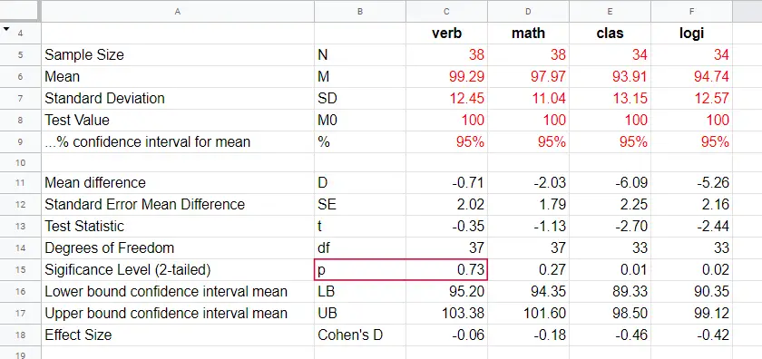
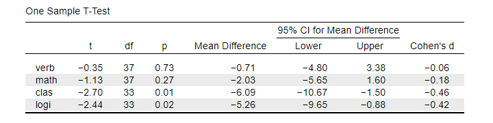
Given \(t\) and \(df\), we can simply look up that the 2-tailed significance level \(p\) = 0.73 in this Googlesheet, partly shown below.
Interpretation
As a rule of thumb, we
reject the null hypothesis if p < 0.05.
We just found that p = 0.73 so we don't reject our null hypothesis: given our sample data, the population mean being 100 is a credible statement.
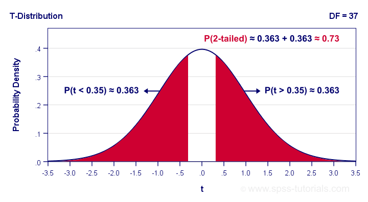
So precisely what does p = 0.73 mean? Well, it means there's a 0.73 (or 73%) probability that t < -0.35 or t > 0.35. The figure below illustrates how this probability results from the sampling distribution, t(37).
Next, remember that t is just a standardized mean difference. For our data, t = -0.35 corresponds to a difference of -0.71 IQ points. Therefore, p = 0.73 means that there's a 0.73 probability of finding an absolute mean difference of at least 0.71 points. Roughly speaking,
the sample mean we found is likely to occur
if the null hypothesis is true.
Effect Size
The only effect size measure for a one-sample t-test is Cohen’s D defined as
$$Cohen's\;D = \frac{M - \mu_0}{SD}$$
For our first IQ test component, this results in
$$Cohen's\;D = \frac{99.29 - 100}{12.45} = -0.06$$
Some general conventions are that
- | Cohen’s D | = 0.20 indicates a small effect size;
- | Cohen’s D | = 0.50 indicates a medium effect size;
- | Cohen’s D | = 0.80 indicates a large effect size.
This means that Cohen’s D = -0.06 indicates a negligible effect size for our first test component. Cohen’s D is completely absent from SPSS except for SPSS 27. However, we can easily obtain it from JASP. The JASP output below shows the effect sizes for all 4 IQ test components.
Note that the last 2 IQ components -clas and logi- almost have medium effect sizes. These are also the 2 components whose means differ significantly from 100: p < 0.05 for both means (third table column).
Confidence Intervals for Means
Our data came up with sample means for our 4 IQ test components. Now, we know that sample means typically differ somewhat from their population counterparts.
So what are likely ranges for the population means we're after?
This is often answered by computing 95% confidence intervals. We'll demonstrate the procedure for our last IQ component, logical reasoning.
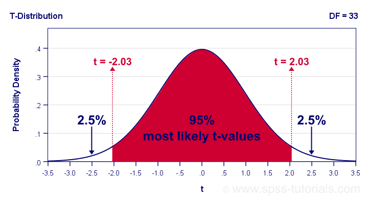
Since we've 34 observations, t follows a t-distribution with df = 33. We'll first look up which t-values enclose the most likely 95% from the inverse t-distribution. We'll do so by typing
=T.INV(0.025,33)
into any cell of a Googlesheet, which returns -2.03. Note that 0.025 is 2.5%. This is because the 5% most unlikely values are divided over both tails of the distribution as shown below.
Now, our t-value of -2.03 estimates that our 95% of our sample means fluctuate between ± 2.03 standard errors denoted by \(SE_{mean}\) For our last IQ component,
$$SE_{mean} = \frac{12.57}{\sqrt34} = 2.16 $$
We now know that 95% of our sample means are estimated to fluctuate between ± 2.03 · 2.16 = 4.39 IQ test points. Last, we combine this fluctuation with our observed sample mean of 94.74:
$$CI_{95\%} = [94.74 - 4.39,94.74 + 4.39] = [90.35,99.12]$$
Note that our 95% confidence interval does not enclose our hypothesized population mean of 100. This implies that we'll reject this null hypothesis at α = 0.05. We don't even need to run the actual t-test for drawing this conclusion.
APA Style Reporting
A single t-test is usually reported in text as in
“The mean for verbal skills did not differ from 100,
t(37) = -0.35, p = 0.73, Cohen’s D = 0.06.”
For multiple tests, a simple overview table as shown below is recommended. We feel that confidence intervals for means (not mean differences) should also be included. Since the APA does not mention these, we left them out for now.
 APA Style Reporting Table Example for One-Sample T-Tests
Right. Well, I can't think of anything else that is relevant regarding the one-sample t-test. If you do, don't be shy. Just write us a comment below. We're always happy to hear from you!
Thanks for reading!
SPSS Paired Samples T-Test Tutorial
A paired samples t-test examines if 2 variables
are likely to have equal population means.
- Paired Samples T-Test Assumptions
- SPSS Paired Samples T-Test Dialogs
- Paired Samples T-Test Output
- Effect Size - Cohen’s D
- Testing the Normality Assumption
Example
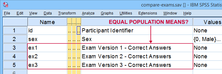
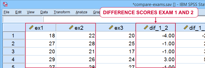
A teacher developed 3 exams for the same course. He needs to know if they're equally difficult so he asks his students to complete all 3 exams in random order. Only 19 students volunteer. Their data -partly shown below- are in compare-exams.sav. They hold the number of correct answers for each student on all 3 exams.
Null Hypothesis
Generally, the null hypothesis for a paired samples t-test is that 2 variables have equal population means. Now, we don't have data on the entire student population. We only have a sample of N = 19 students and sample outcomes tend to differ from population outcomes. So even if the population means are really equal, our sample means may differ a bit. However, very different sample means are unlikely and thus suggest that the population means aren't equal after all. So are the sample means different enough to draw this conclusion? We'll answer just that by running a paired samples t-test on each pair of exams. However, this test requires some assumptions so let's look into those first.
Paired Samples T-Test Assumptions
Technically, a paired samples t-test is equivalent to a one sample t-test on difference scores. It therefore requires the same 2 assumptions. These are
- independent observations;
- normality: the difference scores must be normally distributed in the population. Normality is only needed for small sample sizes, say N < 25 or so.
Our exam data probably hold independent observations: each case holds a separate student who didn't interact with the other students while completing the exams.
Since we've only N = 19 students, we do require the normality assumption. The only way to look into this is actually computing the difference scores between each pair of examns as new variables in our data. We'll do so later on.
At this point, you should carefully inspect your data. At the very least, run some histograms over the outcome variables and see if these look plausible. If necessary, set and count missing values for each variable as well. If all is good, proceed with the actual tests as shown below.
SPSS Paired Samples T-Test Dialogs
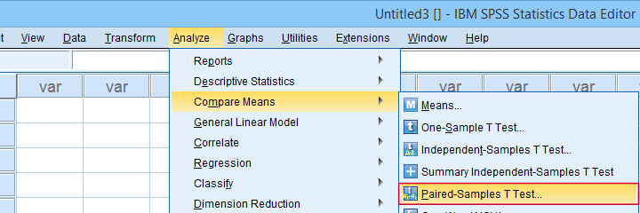
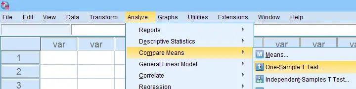
You find the paired samples t-test under
![]()
![]() as shown below.
as shown below.
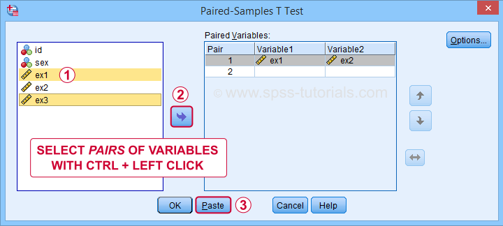
In the dialog below,  select each pair of variables and
  move it to “Paired Variables”. For 3 pairs of variables, you need to do this 3 times.
 Clicking creates the syntax below. We added a shorter alternative to the pasted syntax for which you can bypass the entire dialog. Let's run either version.
Paired Samples T-Test Syntax
T-TEST PAIRS=ex1 ex1 ex2 WITH ex2 ex3 ex3 (PAIRED)
/CRITERIA=CI(.9500)
/MISSING=ANALYSIS.
*Shorter version below results in exact same output.
T-TEST PAIRS=ex1 to ex3
/CRITERIA=CI(.9500)
/MISSING=ANALYSIS.
Paired Samples T-Test Output
SPSS creates 3 output tables when running the test. The last one -Paired Samples Test- shows the actual test results.
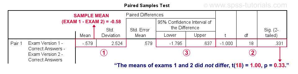
SPSS reports the mean and standard deviation of the difference scores for each pair of variables. The mean is the difference between the sample means. It should be close to zero if the populations means are equal.
The mean difference between exams 1 and 2 is not statistically significant at α = 0.05. This is because ‘Sig. (2-tailed)’ or p > 0.05.
The 95% confidence interval includes zero: a zero mean difference is well within the range of likely population outcomes.
In a similar vein, the second test (not shown) indicates that the means for exams 1 and 3 do differ statistically significantly, t(18) = 2.46, p = 0.025. The same goes for the final test between exams 2 and 3.
Effect Size - Cohen’s D
Our t-tests show that exam 3 has a lower mean score than the other 2 exams. The next question is: are the differences large or small? One way to answer this is computing an effect size measure. For t-tests, Cohen’s D is often used. It's absent from SPSS versions 26 and lower but -if needed- it's easily computed in Excel as shown below.
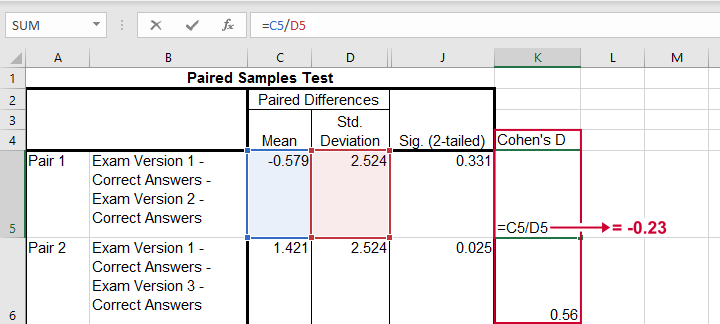
The effect sizes thus obtained are
- d = -0.23 (pair 1) - roughly a small effect;
- d = 0.56 (pair 2) - slightly over a medium effect;
- d = 0.57 (pair 3) - slightly over a medium effect.
Interpretational Issues
Thus far, we compared 3 pairs of exams using 3 t-tests. A shortcoming here is that all 3 tests use the same tiny student sample. This increases the risk that at least 1 test is statistically significant just by chance. There's 2 basic solutions for this:
- apply a Bonferroni correction in order to adjust the significance levels;
- run a repeated measures ANOVA on all 3 exams simultaneously.
If you choose the ANOVA approach, you may want to follow it up with post hoc tests. And these are -guess what?- Bonferroni corrected t-tests again...
Testing the Normality Assumption
Thus far, we blindly assumed that the normality assumption for our paired samples t-tests holds. Since we've a small sample of N = 19 students, we do need this assumption. The only way to evaluate it, is computing the actual difference scores as new variables in our data. We'll do so with the syntax below.
compute dif_1_2 = ex1 - ex2.
compute dif_1_3 = ex1 - ex3.
compute dif_2_3 = ex2 - ex3.
execute.
Result
We can now test the normality assumption by running
- a Shapiro-Wilk test,
- a Kolmogorov-Smirnov test or
- an Anderson-Darling test
on our newly created difference scores. Since we discussed such tests in separate tutorials, we'll limit ourselves to the syntax below.
EXAMINE VARIABLES=dif_1_2 dif_1_3 dif_2_3
/statistics none
/plot npplot.
*Note: difference score between 1 and 2 violates normality assumption.
Result
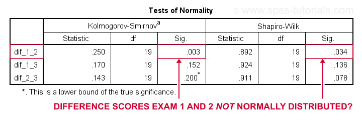
Conclusion: the difference scores between exams 1 and 2 are unlikely to be normally distributed in the population. This violates the normality assumption required by our t-test. This implies that we should perhaps not run a t-test at all on exams 1 and 2. A good alternative for comparing these variables is a Wilcoxon signed-ranks test as this doesn't require any normality assumption.
Last, if you compute difference scores, you can circumvent the paired samples t-tests altogether: instead, you can run one-sample t-tests on the difference scores with zeroes as test values. The syntax below does just that. If you run it, you'll get the exact same results as from the previous paired samples tests.
T-TEST
/TESTVAL=0
/MISSING=ANALYSIS
/VARIABLES=dif_1_2 dif_1_3 dif_2_3
/CRITERIA=CI(.95).
Right, so that'll do for today. Hope you found this tutorial helpful. And as always:
thanks for reading!
Confidence Intervals for Means in SPSS
- Assumptions for Confidence Intervals for Means
- Any Confidence Level - All Cases
- 95% Confidence Level - Separate Groups
- Any Confidence Level - Separate Groups
- Bonferroni Corrected Confidence Intervals
Confidence intervals for means are among the most essential statistics for reporting. Sadly, they're pretty well hidden in SPSS. This tutorial quickly walks you through the best (and worst) options for obtaining them. We'll use adolescents_clean.sav -partly shown below- for all examples.
Assumptions for Confidence Intervals for Means
Computing confidence intervals for means requires
- independent observations and
- normality: our variables must be normally distributed in the population represented by our sample.
1. A visual inspection of our data suggests that each case represents a distinct respondent so it seems safe to assume these are independent observations.
2. Second, the normality assumption is only required for small samples of N < 25 or so. For larger samples, the central limit theorem ensures that the sampling distributions for means, sums and proportions approximate normal distributions. In short,
our example data meet both assumptions.
Any Confidence Level - All Cases I
If we want to analyze all cases as a single group, our best option is the one sample t-test dialog.
The final output will include confidence intervals for the differences between our test value and our sample means. Now, if we use 0 as the test value, these differences will be exactly equal to our sample means.
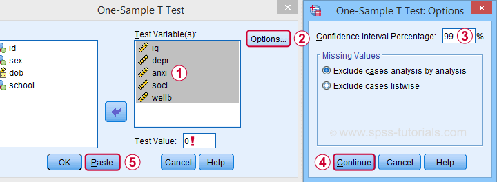
Clicking results in the syntax below. Let's run it.
T-TEST
/TESTVAL=0
/MISSING=ANALYSIS
/VARIABLES=iq depr anxi soci wellb
/CRITERIA=CI(.99).
Result
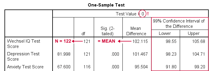
- as long as we use 0 as the test value, mean differences are equal to the actual means. This holds for their confidence intervals as well;
- the table indirectly includes the sample sizes: df = N - 1 and therefore N = df + 1.
Any Confidence Level - All Cases II
An alternative -but worse- option for obtaining these same confidence intervals is from
![]()
![]() We'll discuss these dialogs and their output in a minute under Any Confidence Level - Separate Groups II. They result in the syntax below.
We'll discuss these dialogs and their output in a minute under Any Confidence Level - Separate Groups II. They result in the syntax below.
EXAMINE VARIABLES=iq depr anxi soci wellb
/PLOT NONE
/STATISTICS DESCRIPTIVES
/CINTERVAL 95
/MISSING PAIRWISE /*IMPORTANT!*/
/NOTOTAL.
*Minimal syntax - returns 95% CI's by default.
examine iq depr anxi soci wellb
/missing pairwise /*IMPORTANT!*/.
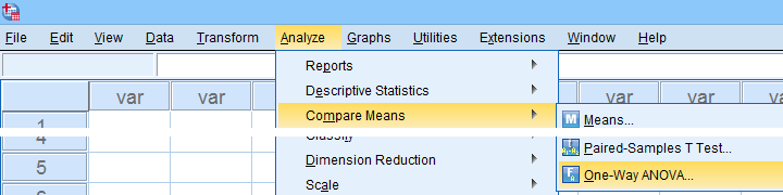
95% Confidence Level - Separate Groups
In many situations, analysts report statistics for separate groups such as male and female respondents. If these statistics include 95% confidence intervals for means, the way to go is the One-Way ANOVA dialog.
Now, sex is a dichotomous variable so we compare these 2 means with a t-test rather than an ANOVA -even though the significance levels are identical for these tests. However, the dialogs below result in a much nicer -and technically correct- descriptives table than the t-test dialogs.
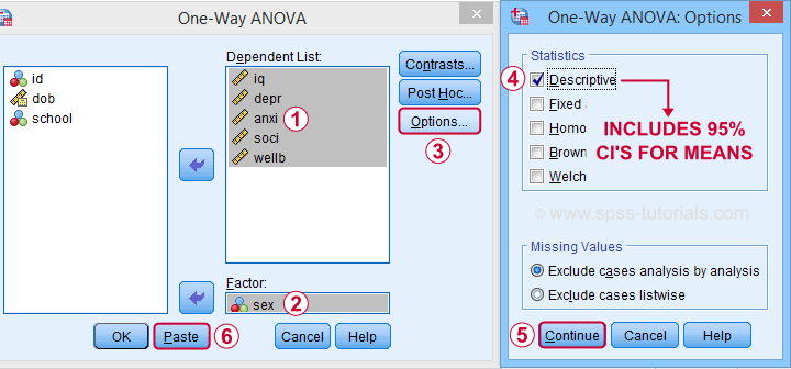
 Descriptives includes 95% CI's for means but other confidence levels aren't available.
 Clicking results in the syntax below. Let's run it.
ONEWAY iq depr anxi soci wellb BY sex
/STATISTICS DESCRIPTIVES .
Result
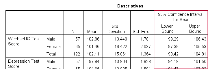
The resulting table has a nice layout that comes pretty close to the APA recommended format. It includes
- sample sizes;
- sample means;
- standard deviations and
- 95% CI's for means.
As mentioned, this method is restricted to 95% CI's. So let's look into 2 alternatives for other confidence levels.
Any Confidence Level - Separate Groups I
So how to obtain other confidence intervals for separate groups? The best option is adding a SPLIT FILE to the One Sample T-Test method. Since we discussed these dialogs and output under Any Confidence Level - All Cases I, we'll now just present the modified syntax.
sort cases by sex.
split file layered by sex.
*Obtain 95% CI's for means of iq to wellb.
T-TEST
/TESTVAL=0
/MISSING=ANALYSIS
/VARIABLES=iq depr anxi soci wellb
/CRITERIA=CI(.95).
*Switch off SPLIT FILE for succeeding output.
split file off.
Any Confidence Level - Separate Groups II
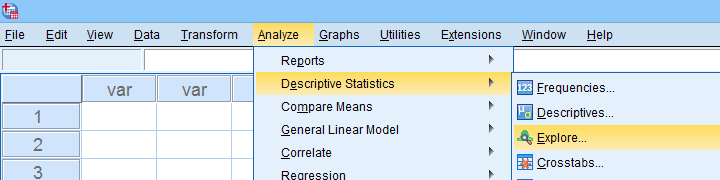
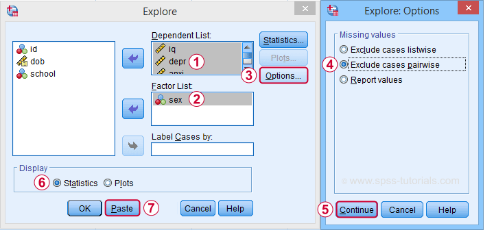
A last option we should mention is the Explore dialog as shown below.
We mostly discuss it for the sake of completeness because
SPSS’ Explore dialog is a real showcase of stupidity
and poor UX design.
Just a few of its shortcomings are that
- you can select “statistics” but not which statistics;
- if you do so, you always get a tsunami of statistics -the vast majority of which you don't want;
- what you probably do want are sample sizes but these are not available;
- the sample sizes that are actually used may be different than you think: in contrast to similar dialogs, Explore uses listwise exclusion of missing values by default;
- what you probably do want, is exclusion of missing values by analysis or variable. This is available but mislabeled “pairwise” exclusion.
- the Explore dialog generates an EXAMINE command so many users think these are 2 separate procedures.
For these reasons, I personally only use Explore for
These tests are under -the very last place you'd expect them.
But anyway, the steps shown below result in confidence intervals for means for males and females separately.
 Clicking generates the syntax below.
EXAMINE VARIABLES=iq depr anxi soci wellb BY sex
/PLOT NONE
/STATISTICS DESCRIPTIVES
/CINTERVAL 95
/MISSING PAIRWISE /*IMPORTANT!*/
/NOTOTAL.
*Minimal syntax - returns 95% CI's by default.
examine iq depr anxi soci wellb by sex
/missing pairwise /*IMPORTANT!*/
/nototal.
Result
Bonferroni Corrected Confidence Intervals
All examples in this tutorial used 5 outcome variables measured on the same sample of respondents. Now, a 95% confidence interval has a 5% chance of not enclosing the population parameter we're after. So for 5 such intervals, there's a (1 - 0.955 =) 0.226 probability that at least one of them is wrong.
Some analysts argue that this problem should be fixed by applying a Bonferroni correction. Some procedures in SPSS have this as an option as shown below.
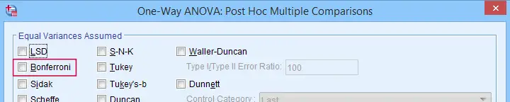
But what about basic confidence intervals? The easiest way is probably to adjust the confidence levels manually by
$$level_{adj} = 100\% - \frac{100\% - level_{unadj}}{N_i}$$
where \(N_i\) denotes the number of intervals calculated on the same sample. So some Bonferroni adjusted confidence levels are
- 95.00% if you calculate 1 (95%) confidence interval;
- 97.50% if you calculate 2 (95%) confidence intervals;
- 98.33% if you calculate 3 (95%) confidence intervals;
- 98.75% if you calculate 4 (95%) confidence intervals;
- 99.00% if you calculate 5 (95%) confidence intervals;
and so on.
Well, I think that should do. I can't think of anything else I could write on this topic. If you do, please throw us a comment below.
Thanks for reading!
Independent Samples T-Test – Quick Introduction
- Independent Samples T-Test - What Is It?
- Null Hypothesis
- Test Statistic
- Assumptions
- Statistical Significance
- Effect Size
Independent Samples T-Test - What Is It?
An independent samples t-test evaluates if 2 populations have equal means on some variable.
If the population means are really equal, then the sample means will probably differ a little bit but not too much. Very different sample means are highly unlikely if the population means are equal. This sample outcome thus suggest that the population means weren't equal after all.
The samples are independent because they don't overlap; none of the observations belongs to both samples simultaneously. A textbook example is male versus female respondents.
Example
Some island has 1,000 male and 1,000 female inhabitants. An investigator wants to know if males spend more or fewer minutes on the phone each month. Ideally, he'd ask all 2,000 inhabitants but this takes too much time. So he samples 10 males and 10 females and asks them. Part of the data are shown below.
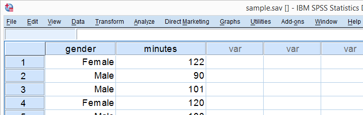
Next, he computes the means and standard deviations of monthly phone minutes for male and female respondents separately. The results are shown below.
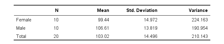
These sample means differ by some (99 - 106 =) -7 minutes: on average, females spend some 7 minutes less on the phone than males. But that's just our tiny samples. What can we say about the entire populations? We'll find out by starting off with the null hypothesis.
Null Hypothesis
The null hypothesis for an independent samples t-test is (usually) that the 2 population means are equal. If this is really true, then we may easily find slightly different means in our samples. So precisely what difference can we expect? An intuitive way for finding out is a simple simulation.
Simulation
I created a fake dataset containing the entire populations of 1,000 males and 1,000 females. On average, both groups spend 103 minutes on the phone with a standard-deviation of 14.5. Note that the null hypothesis of equal means is clearly true for these populations.
I then sampled 10 males and 10 females and computed the mean difference. And then I repeated that process 999 times, resulting in the 1,000 sample mean differences shown below.
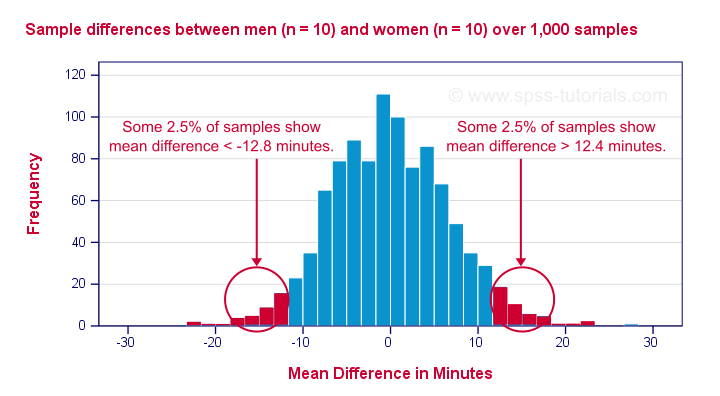
First off, the mean differences are roughly normally distributed. Most of the differences are close to zero -not surprising because the population difference is zero. But what's really interesting is that mean differences between, say, -12.5 and 12.5 are pretty common and make up 95% of my 1,000 outcomes. This suggests that an absolute difference of 12.5 minutes is needed for statistical significance at α = 0.05.
Last, the standard deviation of our 1,000 mean differences -the standard error- is 6.4. Note that some 95% of all outcomes lie between -2 and +2 standard errors of our (zero) mean. This is one of the best known rules of thumb regarding the normal distribution.
Now, an easier -though less visual- way to draw these conclusions is using a couple of simple formulas.
Test Statistic
Again: what is a “normal” sample mean difference if the population difference is zero? First off, this depends on the population standard deviation of our outcome variable. We don't usually know it but we can estimate it with
$$Sw = \sqrt{\frac{(n_1 - 1)\;S^2_1 + (n_2 - 1)\;S^2_2}{n_1 + n_2 - 2}}$$
in which \(Sw\) denotes our estimated population standard deviation.
For our data, this boils down to
$$Sw = \sqrt{\frac{(10 - 1)\;224 + (10 - 1)\;191}{10 + 10 - 2}} ≈ 14.4$$
Second, our mean difference should fluctuate less -that is, have a smaller standard error- insofar as our sample sizes are larger. The standard error is calculated as
$$Se = Sw\sqrt{\frac{1}{n_1} + \frac{1}{n_2}}$$
and this gives us
$$Se = 14.4\; \sqrt{\frac{1}{10} + \frac{1}{10}} ≈ 6.4$$
If the population mean difference is zero, then -on average- the sample mean difference will be zero as well. However, it will have a standard deviation of 6.4. We can now just compute a z-score for the sample mean difference but -for some reason- it's called T instead of Z:
$$T = \frac{\overline{X}_1 - \overline{X}_2}{Se}$$
which, for our data, results in
$$T = \frac{99.4 - 106.6}{6.4} ≈ -1.11$$
Right, now this is our test statistic: a number that summarizes our sample outcome with regard to the null hypothesis. T is basically the standardized sample mean difference; T = -1.11 means that our difference of -7 minutes is roughly 1 standard deviation below the average of zero.
Assumptions
Our t-value follows a t distribution but only if the following assumptions are met:
- Independent observations or, precisely, independent and identically distributed variables.
- Normality: the outcome variable follows a normal distribution in the population. This assumption is not needed for reasonable sample sizes (say, N > 25).
- Homogeneity: the outcome variable has equal standard deviations in our 2 (sub)populations. This is not needed if the sample sizes are roughly equal. Levene's test is sometimes used for testing this assumption.
If our data meet these assumptions, then T follows a t-distribution with (n1 + n2 -2) degrees of freedom (df). In our example, df = (10 + 10 - 2) = 18. The figure below shows the exact distribution. Note that we need an absolute t-value of 2.1 for 2-tailed significance at α = 0.05.
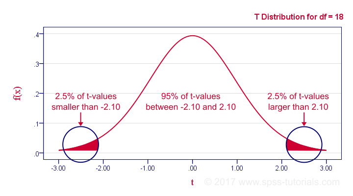
Minor note: as df becomes larger, the t-distribution approximates a standard normal distribution. The difference is hardly noticeable if df > 15 or so.
Statistical Significance
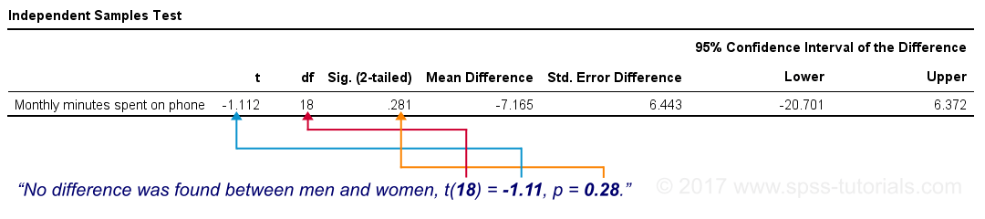
Last but not least, our mean difference of -7 minutes is not statistically significant: t(18) = -1.11, p ≈ 0.28. This means we've a 28% chance of finding our sample mean difference -or a more extreme one- if our population means are really equal; it's a normal outcome that doesn't contradict our null hypothesis.
Our final figure shows these results as obtained from SPSS.
Effect Size
Finally, the effect size measure that's usually preferred is Cohen’s D, defined as
$$D = \frac{\overline{X}_1 - \overline{X}_2}{Sw}$$
in which \(Sw\) is the estimated population standard deviation we encountered earlier. That is,
Cohen’s D is the number of standard deviations between the 2 sample means.
So what is a small or large effect? The following rules of thumb have been proposed:
- D = 0.20 indicates a small effect;
- D = 0.50 indicates a medium effect;
- D = 0.80 indicates a large effect.
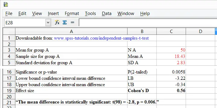
Cohen’s D is painfully absent from SPSS except for SPSS 27. However, you can easily obtain it from Cohens-d.xlsx. Just fill in 2 sample sizes, means and standard deviations and its formulas will compute everything you need to know.
Thanks for reading!
SPSS Independent Samples T-Test
A newly updated, ad-free video version of this tutorial
is included in our SPSS beginners course.
- Assumptions
- Independent Samples T-Test Flowchart
- Independent Samples T-Test Dialogs
- Output I - Significance Levels
- Output II - Effect Size
- APA Reporting - Tables & Text
Introduction & Example Data
An independent samples t-test examines if 2 populations
have equal means on some quantitative variable.
For instance, do children from divorced versus non-divorced parents have equal mean scores on psychological tests? We'll walk you through using divorced.sav, part of which is shown below.
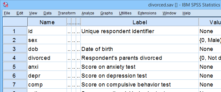
First off, I'd like to shorten some variable labels with the syntax below. Doing so prevents my tables from becoming too wide to fit the pages in my final thesis.
variable labels
anxi 'Anxiety'
depr 'Depression'
comp 'Compulsive Behavior'
anti 'Antisocial Behavior'.
Let's now take a quick look at what's in our data in the first place. Does everything look plausible? Are there any outliers or missing values? I like to find out by running some quick histograms from the syntax below.
frequencies anxi to anti
/format notables
/histogram.
Result
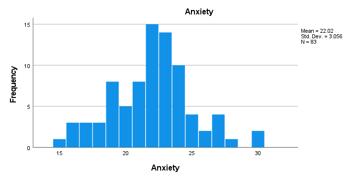
- First, note that all frequency distributions look plausible: we don't see anything weird or unusual.
- Also, none of our histograms show any clear outliers on any of our variables.
- Finally, note that N = 83 for each variable. Since this is our total sample size, this implies that none of them contain any missing values.
After this quick inspection, I like to create a table with sample sizes, means & standard deviations of all dependent variables for both groups separately.
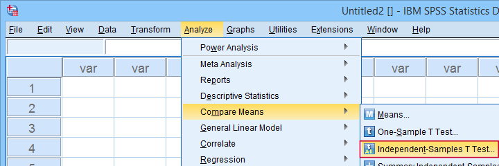
The best way to do so is from
![]()
![]() but the syntax is so simple that just typing it is faster:
but the syntax is so simple that just typing it is faster:
means anxi to anti by divorced
/cells count mean stddev.
Result
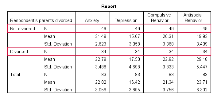
- Note that n = 49 (parents not divorced) and n = 34 (parents divorced) for all dependent variables.
- Also note that children from divorced parents have slightly higher mean scores on most tests. The difference on antisocial behavior (final column) is especially large.
Now, the big question is:
can we conclude from these sample differences
that the entire populations are also different?
An independent samples t-test will answer precisely that. It does, however, require some assumptions.
Assumptions
- independent observations. This often holds if each row of data represents a different person.
- Normality: the dependent variable must follow a normal distribution in each subpopulation. This is not needed if both n ≥ 25 or so.
- Homogeneity of variances: both subpopulations must have equal variances on the dependent variable. This is not needed if both sample sizes are roughly equal.
If sample sizes are not roughly equal, then Levene's test may be used to test if homogeneity is met. If that's not the case, then you should report adjusted results. These are shown in the SPSS t-test output under “equal variances not assumed”.
More generally, this procedure is known as the Welch test and also applies to ANOVA as covered in SPSS ANOVA - Levene’s Test “Significant”.
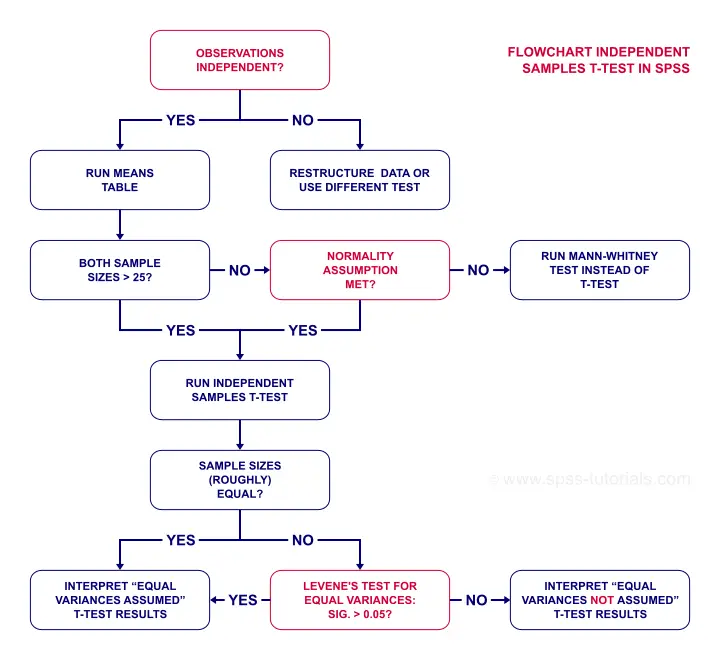
Now, if that's a little too much information, just try and follow the flowchart below.
Independent Samples T-Test Flowchart
Independent Samples T-Test Dialogs
First off, let's navigate to
![]()
![]() as shown below.
as shown below.
Next, we fill out the dialog as shown below.
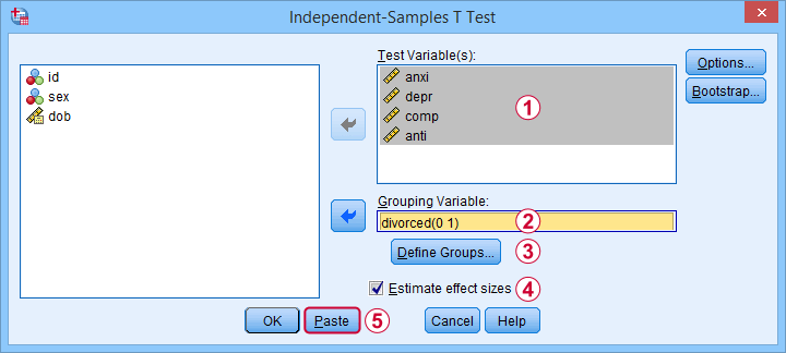
 Sadly, the effect sizes are only available in SPSS version 27 and higher. Since they're very useful, try and upgrade if you're still on SPSS 26 or older.
Anyway, completing these steps results in the syntax below. Let's run it.
T-TEST GROUPS=divorced(0 1)
/MISSING=ANALYSIS
/VARIABLES=anxi depr comp anti
/ES DISPLAY(TRUE)
/CRITERIA=CI(.95).
Output I - Significance Levels
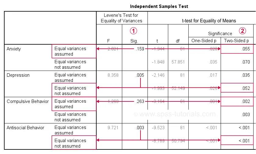
As previously discussed, each dependent variable has 2 lines of results. Which line to report depends on  Levene’s test because our sample sizes are not (roughly) equal:
- if Levene’s test “Sig” or p ≥ .05, then report the “Equal variances assumed”
 t-test results.
 - otherwise, report the “Equal variances not assumed” t-test results.
Following this procedure, we conclude that the mean differences on anxiety (p = .055) and depression (p = .052) are not statistically significant.
The differences on compulsive behavior (p = .002) and antisocial behavior (p < .001), however are both highly “significant”.
This last finding means that our sample differences are highly unlikely if our populations have exactly equal means. The output also includes the mean differences and their confidence intervals.
For example, the mean difference on anxiety is -1.30 points on the anxiety test. But what we don't know, is: should we consider this a small, medium or large difference? We'll answer just that by standardizing our mean differences into effect size measures.
Output II - Effect Size
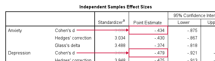
The most common effect size measure for t-tests is Cohen’s D, which we find under “point estimate” in the effect sizes table (only available for SPSS version 27 onwards).
Some general rules of thumb are that
- |d| = 0.20 indicates a small effect;
- |d| = 0.50 indicates a medium effect;
- |d| = 0.80 indicates a large effect.
Like so, we could consider d = -0.43 for our anxiety test roughly a medium effect of divorce and so on.
APA Reporting - Tables & Text
The figure below shows the exact APA style table for reporting the results obtained during this tutorial.
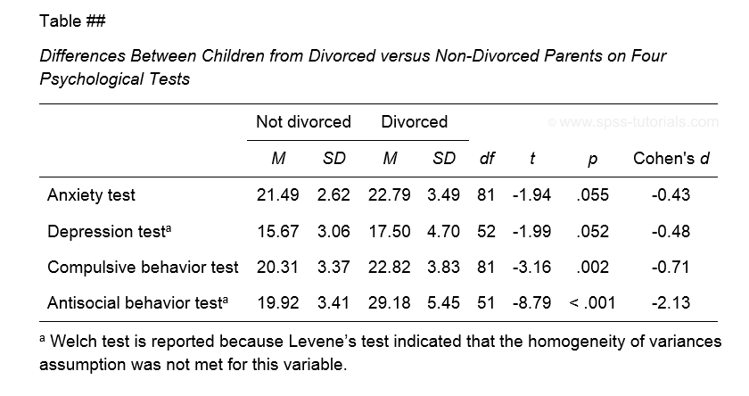
Minor note: if all tests have equal df (degrees of freedom), you may omit this column. In this case, add df to the column header for t as in t(81).
This table was created by combining results from 3 different SPSS output tables in Excel. This doesn't have to be a lot of work if you master a couple of tricks. I hope to cover these in a separate tutorial some time soon.
If you prefer reporting results in text format, follow the example below.
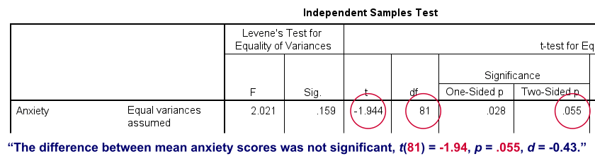
Note that d = -0.43 refers to Cohen’s D here, which is obtained from a separate table as previously discussed.
Final Notes
Most textbooks will tell you to
- use an independent samples t-test for comparing means between 2 subpopulations and
- use ANOVA for comparing means among 3+ subpopulations.
So what happens if we run ANOVA instead of t-tests on the 2 groups in our data? The syntax below does just that.
ONEWAY anxi depr comp anti BY divorced
/ES=OVERALL
/STATISTICS HOMOGENEITY WELCH
/MISSING ANALYSIS
/CRITERIA=CILEVEL(0.95).
Those who ran this syntax will quickly see that most results are identical. This is because an independent samples t-test is a special case of ANOVA. There's 2 important differences, though:
- ANOVA comes up with a single p-value which is identical to p(2-tailed) from the corresponding t-test;
- the effect size for ANOVA is (partial) eta squared rather than Cohen’s D.
This raises an important question:
why do we report different measures for comparing
2 rather than 3+ groups?
My answer: we shouldn't. And this implies that we should
- always report p(2-tailed) for t-tests, never p(1-tailed);
- report eta-squared as the effect size for t-tests and abandon Cohen’s D.
Thanks for reading!
What is a Dichotomous Variable?
A dichotomous variable is a variable that contains precisely two distinct values. Let's first take a look at some examples for illustrating this point. Next, we'll point out why distinguishing dichotomous from other variables makes it easier to analyze your data and choose the appropriate statistical test.
Examples
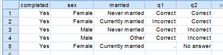
Regarding the data in the screenshot:
- completed is not a dichotomous variable. It contains only one distinct value and we therefore call it a constant rather than a variable.
- sex is a dichotomous variable as it contains precisely 2 distinct values.
- married is not a dichotomous variable: it contains 3 distinct values. It would be dichotomous if we just distinguished between currently married and currently unmarried.
- q1 is a dichotomous variable: since empty cells (missing values) are always excluded from analyses, we have two distinct values left.
- q2 is a dichotomous variable if we exclude the “no answer” category from analysis and not dichotomous otherwise.
Dichotomous Variables - What Makes them Special?
Dichotomous are the simplest possible variables. The point here is that -given the sample size- the frequency distribution of a dichotomous variable can be exactly described with a single number: if we've 100 observations on sex and 45% is male, then we know all there is to know about this variable.
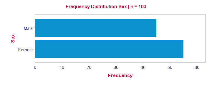
Note that this doesn't hold for other categorical variables: if we know that 45% of our sample (n = 100) has brown eyes, then we don't know the percentages of blue eyes, green eyes and so forth. That is, we can't describe the exact frequency distribution with one single number.
Something similar holds for metric variables: if we know the average age of our sample (n = 100) is precisely 25 years old, then we don't know the variance, skewness, kurtosis and so on needed for drawing a histogram.
Dichotomous Variables are both Categorical and Metric
Choosing the right data analysis techniques becomes much easier if we're aware of the measurement levels of the variables involved. The usual classification involves categorical (nominal, ordinal) and metric (interval, ratio) variables. Dichotomous variables, however, don't fit into this scheme because they're both categorical and metric.
This odd feature (which we'll illustrate in a minute) also justifies treating dichotomous variables as a separate measurement level.
Dichotomous Outcome Variables
Some research questions involve dichotomous dependent (outcome) variables. If so, we use proportions or percentages as descriptive statistics for summarizing such variables. For instance, people may or may consider buying a new car in 2017. We might want to know the percentage of people who do. This question is answered with either a binomial test or a z-test for one proportion.
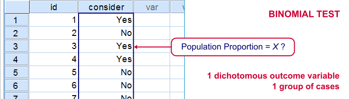
The aforementioned tests -and some others- are used exclusively for dichotomous dependent variables. They are among the most widely used (and simplest) stasticical tests around.
Dichotomous Input Variables
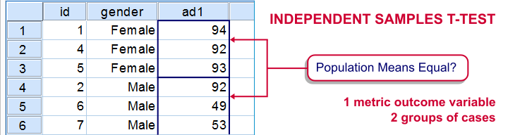
An example of a test using a dichotomous independent (input) variable is the independent samples t-test, illustrated below.
In this test, the dichotomous variable defines groups of cases and hence is used as a categorical variable. Strictly, the independent-samples t-test is redundant because it's equivalent to a one-way ANOVA. However, the independent variable holding only 2 distinct values greatly simplifies the calculations involved. This is why this test is treated separately from the more general ANOVA in most text books.
Those familiar with regression may know that the predictors (or independent variables) must be metric or dichotomous. In order to include a categorical predictor, it must be converted to a number of dichotomous variables, commonly referred to as dummy variables.
This illustrates that in regression, dichotomous variables are treated as metric rather than categorical variables.
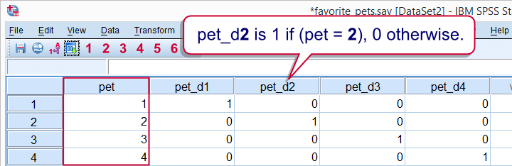
Dichotomizing Variables
Last but not least, a distinction is sometimes made between naturally dichotomous variables and unnaturally dichotomous variables. A variable is naturally dichotomous if precisely 2 values occur in nature (sex, being married or being alive). If a variable holds precisely 2 values in your data but possibly more in the real world, it's unnaturally dichotomous.
Creating unnaturally dichotomous variables from non dichotomous variables is known as dichotomizing. The final screenshot illustrates a handy but little known trick for doing so in SPSS.

I hope you found this tutorial helpful. Thanks for reading!
Z-Scores – What and Why?
Quick Definition
Z-scores are scores that have mean = 0
and standard deviation = 1.
Z-scores are also known as standardized scores because they are scores that have been given a common standard. This standard is a mean of zero and a standard deviation of 1.
Contrary to what many people believe, z-scores are not necessarily normally distributed.
Z-Scores - Example
A group of 100 people took some IQ test. My score was 5. So is that good or bad? At this point, there's no way of telling because we don't know what people typically score on this test. However, if my score of 5 corresponds to a z-score of 0.91, you'll know it was pretty good: it's roughly a standard deviation higher than the average (which is always zero for z-scores).
What we see here is that standardizing scores facilitates the interpretation of a single test score. Let's see how that works.
Scores - Histogram
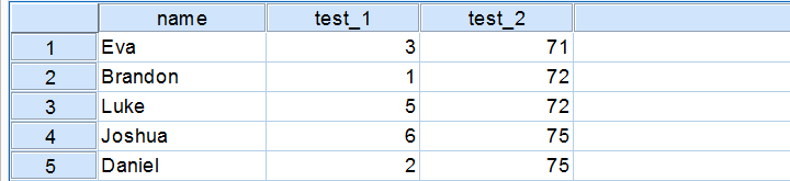
A quick peek at some of our 100 scores on our first IQ test shows a minimum of 1 and a maximum of 6. However, we'll gain much more insight into these scores by inspecting their histogram as shown below.
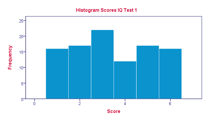
The histogram confirms that scores range from 1 through 6 and each of these scores occurs about equally frequently. This pattern is known as a uniform distribution and we typically see this when we roll a die a lot of times: numbers 1 through 6 are equally likely to come up. Note that these scores are clearly not normally distributed.
Z-Scores - Standardization
We suggested earlier on that giving scores a common standard of zero mean and unity standard deviation facilitates their interpretation. We can do just that by
- first subtracting the mean over all scores from each individual score and
- then dividing each remainder by the standard deviation over all scores.
These two steps are the same as the following formula:
$$Z_x = \frac{X_i - \overline{X}}{S_x}$$
As shown by the table below, our 100 scores have a mean of 3.45 and a standard deviation of 1.70.
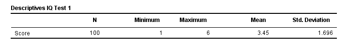 By entering these numbers into the formula, we see why a score of 5 corresponds to a z-score of 0.91:
$$Z_x = \frac{5 - 3.45}{1.70} = 0.91$$
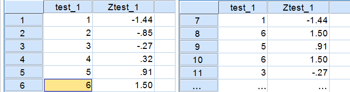
In a similar vein, the screenshot below shows the z-scores for all distinct values of our first IQ test added to the data.
Z-Scores - Histogram
In practice, we obviously have some software compute z-scores for us. We did so and ran a histogram on our z-scores, which is shown below.
 If you look closely, you'll notice that the z-scores indeed have a mean of zero and a standard deviation of 1. Other than that, however, z-scores follow the exact same distribution as original scores. That is, standardizing scores doesn't make their distribution more “normal” in any way.
What's a Linear Transformation?
Z-scores are linearly transformed scores. What we mean by this, is that if we run a scatterplot of scores versus z-scores, all dots will be exactly on a straight line (hence, “linear”). The scatterplot below illustrates this. It contains 100 points but many end up right on top of each other.
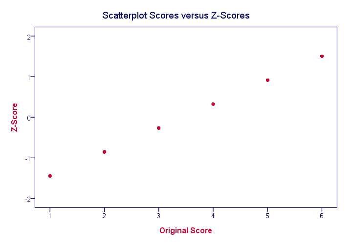
In a similar vein, if we had plotted scores versus squared scores, our line would have been curved; in contrast to standardizing, taking squares is a non linear transformation.
Z-Scores and the Normal Distribution
We saw earlier that standardizing scores doesn't change the shape of their distribution in any way; distribution don't become any more or less “normal”. So why do people relate z-scores to normal distributions?
The reason may be that many variables actually do follow normal distributions. Due to the central limit theorem, this holds especially for test statistics. If a normally distributed variable is standardized, it will follow a standard normal distribution.
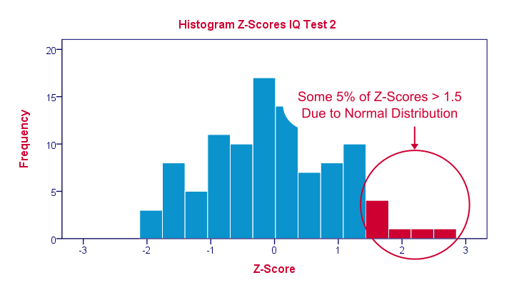
This is a common procedure in statistics because values that (roughly) follow a standard normal distribution are easily interpretable. For instance, it's well known that some 2.5% of values are larger than two and some 68% of values are between -1 and 1.
The histogram below illustrates this: if a variable is roughly normally distributed, z-scores will roughly follow a standard normal distribution. For z-scores, it always holds (by definition) that a score of 1.5 means “1.5 standard deviations higher than average”. However, if a variable also follows a standard normal distribution, then we also know that 1.5 roughly corresponds to the 95th percentile.
Z-Scores in SPSS
SPSS users can easily add z-scores to their data by using a DESCRIPTIVES command as in
descriptives test_1 test_2/save.
in which “save” means “save z-scores as new variables in my data”. For more details, see z-scores in SPSS.
SPSS One Sample T-Test Tutorial
Also see One-Sample T-Test - Quick Tutorial & Example.
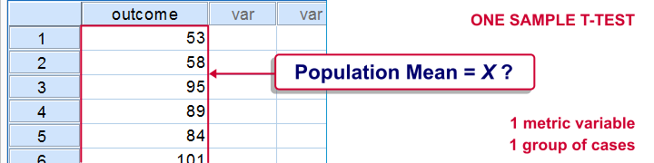
SPSS one-sample t-test tests if the mean of a single quantitative variable is equal to some hypothesized population value. The figure illustrates the basic idea.
SPSS One Sample T-Test - Example
A scientist from Greenpeace believes that herrings in the North Sea don't grow as large as they used to. It's well known that - on average - herrings should weigh 400 grams. The scientist catches and weighs 40 herrings, resulting in herrings.sav. Can we conclude from these data that the average herring weighs less than 400 grams? We'll open the data by running the syntax below.
cd 'd:downloaded'. /*or wherever data file is located.
*2. Open data.
get file 'herrings.sav'.
1. Quick Data Check
Before we run any statistical tests, we always first want to have a basic idea of what the data look like. A fast way for doing so is taking a look at the histogram for body_weight. If we generate it by using FREQUENCIES, we'll get some helpful summary statistics in our chart as well.The required syntax is so simple that we won't bother about clicking through the menu here. We added /FORMAT NOTABLE to the command in order to suppress the actual frequency table; right now, we just want a histogram and some summary statistics.
frequencies body_weight
/format notable
/histogram.

There are no very large or very small values for body_weight. The data thus look plausible. N = 40 means that the histogram is based on 40 cases (our entire sample). This tells us that there are no missing values. The mean weight is around 370 grams, which is 30 grams lower than the hypothesized 400 grams. The question is now: “if the average weight in the population is 400 grams, then what's the chance of finding a mean weight of only 370 grams in a sample of n = 40?”
2. Assumptions One Sample T-Test
Results from statistical procedures can only be taken seriously insofar as relevant assumptions are met. For a one-sample t-test, these are
- independent and identically distributed variables (or, less precisely, “independent observations”);
- normality: the test variable is normally distributed in the population;
Assumption 1 is beyond the scope of this tutorial. We assume it's been met by the data. The normality assumption not holding doesn't really affect the results for reasonable sample sizes (say, N > 30).
3. Run SPSS One-Sample T-Test

The screenshot walks you through running an SPSS one-sample t-test. Clicking results in the syntax below.
T-TEST
/TESTVAL=400
/MISSING=ANALYSIS
/VARIABLES=body_weight
/CRITERIA=CI(.95).
4. SPSS One-Sample T-Test Output

We'll first turn our attention to the One-Sample Statistics table. We already saw most of these statistics in our histogram but this table comes in a handier format for reporting these results.

The actual t-test results are found in the One-Sample Test table.
 -
-  The t value and its degrees of freedom (df) are not immediately interesting but we'll need them for reporting later on.
 The p value, denoted by “Sig. (2-tailed)” is .02; if the population mean is exactly 400 grams, then there's only a 2% chance of finding the result we did. We usually reject the null hypothesis if p < .05. We thus conclude that herrings do not weight 400 grams (but probably less than that).
It's important to notice that the p value of .02 is 2-tailed. This means that the p value consists of a 1% chance for finding a difference < -30 grams and another 1% chance for finding a difference > 30 grams.
 The Mean Difference is simply the sample mean minus the hypothesized mean (369.55 - 400 = -30.45). We could have calculated it ourselves from previously discussed results.
5. Reporting a One-Sample T-Test
Regarding descriptive statistics, the very least we should report, is the mean, standard deviation and N on which these are based. Since these statistics don't say everything about the data, we personally like to include a histogram as well. We may report the t-test results by writing “we found that, on average, herrings weighed less than 400 grams; t(39) = -2.4, p = .020.”