Mahalanobis Distances in SPSS – A Quick Guide
- Summary
- Mahalanobis Distances - Basic Reasoning
- Mahalanobis Distances - Formula and Properties
- Finding Mahalanobis Distances in SPSS
- Critical Values Table for Mahalanobis Distances
- Mahalanobis Distances & Missing Values
Summary
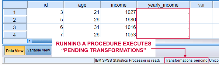
In SPSS, you can compute (squared) Mahalanobis distances as a new variable in your data file. For doing so, navigate to
![]()
![]() and open the “Save” subdialog as shown below.
and open the “Save” subdialog as shown below.
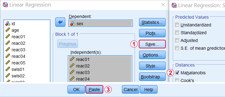
Keep in mind here that Mahalanobis distances are computed only over the independent variables. The dependent variable does not affect them unless it has any missing values. In this case, the situation becomes rather complicated as I'll cover near the end of this article.
Mahalanobis Distances - Basic Reasoning
Before analyzing any data, we first need to know if they're even plausible in the first place. One aspect of doing so is checking for outliers: observations that are substantially different from the other observations. One approach here is to inspect each variable separately and the main options for doing so are
- inspecting histograms;
- inspecting boxplots or
- inspecting z-scores.
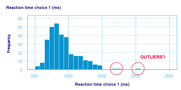
Now, when analyzing multiple variables simultaneously, a better alternative is to check for multivariate outliers: combinations of scores on 2(+) variables that are extreme or unusual. Precisely how extreme or unusual a combination of scores is, is usually quantified by their Mahalanobis distance.
The basic idea here is to add up how much each score differs from the mean while taking into account the (Pearson) correlations among the variables. So why is that a good idea? Well, let's first take a look at the scatterplot below, showing 2 positively correlated variables.
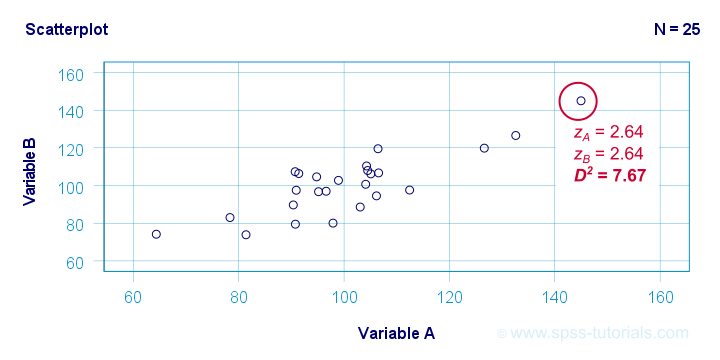
The highlighted observation has rather high z-scores on both variables. However, this makes sense: a positive correlation means that cases scoring high on one variable tend to score high on the other variable too. The (squared) Mahalanobis distance D2 = 7.67 and this is well within a normal range.
So let's now compare this to the second scatterplot shown below.
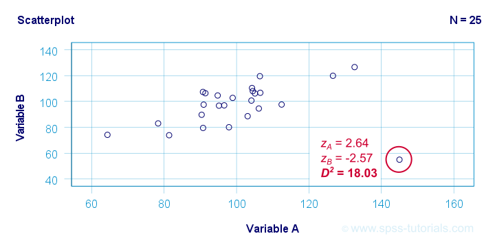
The highlighted observation has a rather high z-score on variable A but a rather low one on variable B. This is highly unusual for variables that are positively correlated. Therefore, this observation is a clear multivariate outlier because its (squared) Mahalanobis distance D2 = 18.03, p < .0005. Two final points on these scatterplots are the following:
- the (univariate) z-scores fail to detect that the highlighted observation in the second scatterplot is highly unusual;
- this observation has a huge impact on the correlation between the variables and is thus an influential data point. Again, this is detected by the (squared) Mahalanobis distance but not by z-scores, histograms or even boxplots.
Mahalanobis Distances - Formula and Properties
Software for applied data analysis (including SPSS) usually computes squared Mahalanobis distances as
\(D^2_i = (\mathbf{x_i} - \mathbf{\overline{x}})'\;\mathbf{S}^{-1}\;(\mathbf{x_i} - \overline{\mathbf{x}})\)
where
- \(D^2\) denotes the squared Mahalanobis distance for case \(i\);
- \(\mathbf{x_i}\) denotes the vector of scores for case \(i\);
- \(\mathbf{\overline{x}}\) denotes the vector of means (centroid) over all cases;
- \(S\) denotes the covariance matrix over all variables.
Some basic properties are that
- Mahalanobis distances can (theoretically) range from zero to infinity;
- Mahalanobis distances are standardized: they are scale independent so they are unaffected by any linear transformations to the variables they're computed on;
- Mahalanobis distances for a single variable are equal to z-scores;
- squared Mahalanobis distances computed over k variables follow a χ2-distribution with df = k under the assumption of multivariate normality.
Finding Mahalanobis Distances in SPSS
In SPSS, you can use the linear regression dialogs to compute squared Mahalanobis distances as a new variable in your data file. For doing so, navigate to
![]()
![]() and open the “Save” subdialog as shown below.
and open the “Save” subdialog as shown below.
Again, Mahalanobis distances are computed only over the independent variables. Although this is in line with most text books, it makes more sense to me to include the dependent variable as well. You could do so by
- adding the actual dependent variable to the independent variables and
- temporarily using an alternative dependent variable that is neither a constant, nor has any missing values.
Finally, if you've any missing values on either the dependent or any of the independent variables, things get rather complicated. I'll discuss the details at the end of this article.
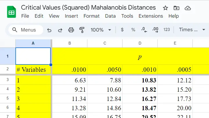
Critical Values Table for Mahalanobis Distances
After computing and inspecting (squared) Mahalanobis distances, you may wonder: how large is too large? Sadly, there's no simples rule of thumb here but most text books suggest that (squared) Mahalanobis distances for which p < .001 are suspicious for reasonable sample sizes. Since p also depends on the number of variables involved, we created a handy overview table in this Googlesheet, partly shown below.
Mahalanobis Distances & Missing Values
Missing values on either the dependent or any of the independent variables may affect Mahalanobis distances. Precisely when and how depends on which option you choose for handling missing values in the linear regression dialogs as shown below.
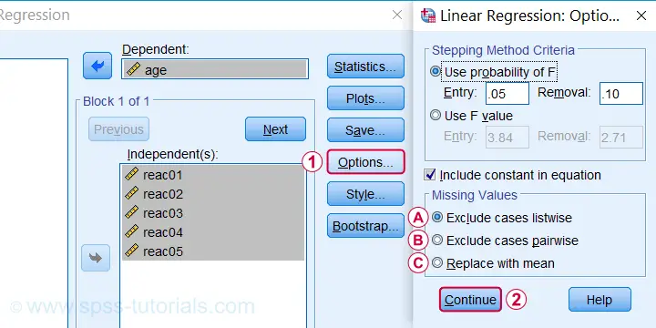
 If you select listwise exclusion,
- Mahalanobis distances are computed for all cases that have zero missing values on the independent variables;
- missing values on the dependent variable may affect the Mahalanobis distances. This is because these are based on the listwise complete covariance matrix over the dependent as well as the independent variables.
 If you select pairwise exclusion,
- Mahalanobis distances are computed for all cases that have zero missing values on the independent variables;
- missing values on the dependent variable do not affect the Mahalanobis distances in any way.
 If you select replace with mean,
- missing values on the dependent and independent variables are replaced with the (variable) means before SPSS proceeds with any further computations;
- Mahalanobis distances are computed for all cases, regardless any missing values;
- \(D^2\) = 0 for cases having missing values on all independent variables. This makes sense because \(\mathbf{x_i} - \mathbf{\overline{x}}\) results in a vector of zeroes after replacing all missing values by means.
References
- Hair, J.F., Black, W.C., Babin, B.J. et al (2006). Multivariate Data Analysis. New Jersey: Pearson Prentice Hall.
- Warner, R.M. (2013). Applied Statistics (2nd. Edition). Thousand Oaks, CA: SAGE.
- Pituch, K.A. & Stevens, J.P. (2016). Applied Multivariate Statistics for the Social Sciences (6th. Edition). New York: Routledge.
- Field, A. (2013). Discovering Statistics with IBM SPSS Statistics. Newbury Park, CA: Sage.
- Howell, D.C. (2002). Statistical Methods for Psychology (5th ed.). Pacific Grove CA: Duxbury.
- Agresti, A. & Franklin, C. (2014). Statistics. The Art & Science of Learning from Data. Essex: Pearson Education Limited.
How to Convert String Variables into Numeric Ones?
Introduction & Practice Data File
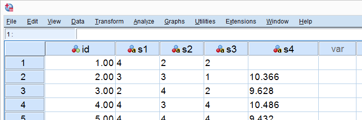
Converting an SPSS string variable into a numeric one is simple. However, there's a huge pitfall that few people are aware of: string values that can't be converted into numbers result in system missing values without SPSS throwing any error or warning.
This can mess up your data without you being aware of it. Don't believe me? I'll demonstrate the problem -and the solution- on convert-strings.sav, part of which is shown below.
SPSS Strings to Numeric - Wrong Way
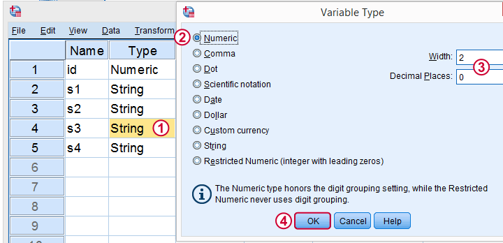
First off, you can convert a string into a numeric variable in variable view as shown below.
Now, I never use this method myself because
- I can't apply it to many variables at once, so it may take way more effort than necessary;
- it doesn't generate any syntax: there's no button and nothing's appended to my journal file;
- it can mess up the data. However, there's remedies for that.
So What's the Problem?
Well, let's do it rather than read about it. We'll
- set empty cells as user missing values for s3;
- convert s3 to numeric in variable view;
- run descriptives on the result.
missing values s3 ('').
*Inspect frequency table for s3.
frequencies s3.
*Now manually convert s3 to numeric under variable view.
*Inspect result.
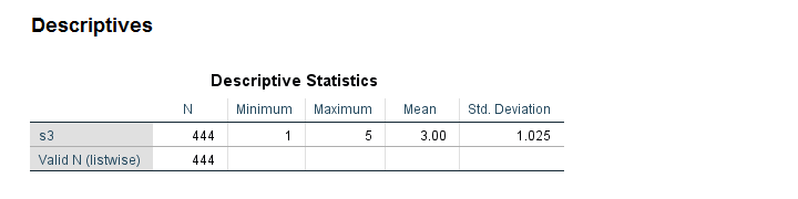
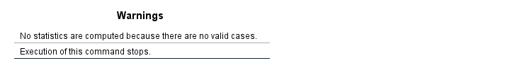
descriptives s3.
*N = 444 instead of 459. That is, 15 values failed to convert and we've no clue why.
Result
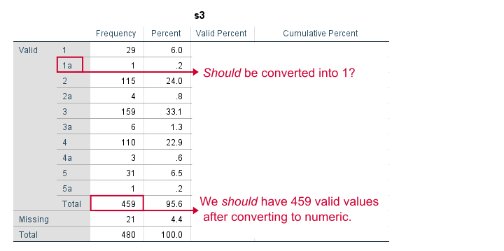
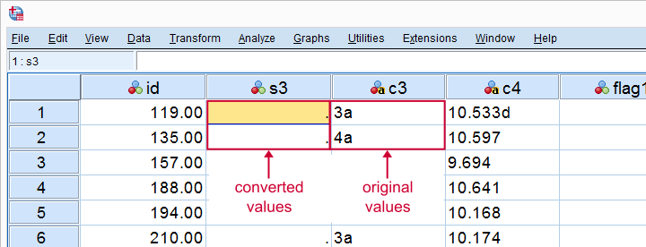
Note that some values in our string variable have been flagged with “a”. We probably want these to be converted into numbers. We have 459 valid values (non empty cells).
After converting our variable to numeric, we ran some descriptives. Note that we only have N = 444. Apparently, 15 values failed to convert -probably not what we want. And we usually won't notice this problem because we don't get any warning or error.
Conversion Failures - Simplest Solution
Right, so how can we perform the conversion safely? Well, we just
- inspected frequency tables: how many non empty values do we have before the conversion?
- converted our variable(s) to numeric;
- inspected N in a descriptive statistics after the conversion. If N is lower than the number of non empty string values (frequencies before conversion), then something may be wrong.
In our first example, the frequency table already suggested we must remove the “a” from all values before converting the variable. We'll do just that in a minute.
Although safe, I still think this method is too much work, especially for multiple variables. Let's speed things up by using some handy syntax.
SPSS - String to Numeric with Syntax
The fastest way to convert string variables into numeric ones is with the ALTER TYPE command.This requires SPSS version 16 or over. For SPSS 15 or below, use the NUMBER function. It allows us to convert many variables with a single line of syntax.
The syntax below converts all string variables in one go. We then check a descriptives table. If we don't have any system missing values, we're done.
SPSS ALTER TYPE Example
*Convert all variables in one go.
alter type s1 to s3 (f1) s4 (f6.3).
*Inspect descriptives.
descriptives s1 to s4.
Note: using alter type s1 to s4 (f1). will also work but the decimal places for s4 won't be visible. This is why we set the correct f format: f6.3 means 6 characters including the decimal separator and 3 decimal places as in 12.345. Which is the format of our string values.
Result
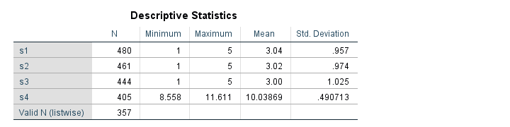
Since we've 480 cases in our data, we're done for s1. However, the other 3 variables contain system missings so we need to find out why. Since we can't undo the operation, let's close our data without saving and reopen it.
Solution 2: Copy String Variables Before Conversion
Things now become a bit more technical. However, readers who struggle their way through will learn a very efficient solution that works for many other situations too. We'll basically
- copy all string variables;
- convert all string variables;
- compare the original to the converted variables.
Precisely, we'll flag non empty string values that are system missing after the conversion. As these are at least suspicious, we'll call those conversion failures. This may sound daunting but it's perfectly doable if we use the right combination of commands. Those are mainly STRING, RECODE, DO REPEAT and IF.
Copy and Convert Several String Variables
*Copy all string variables.
string c1 to c4 (a7).
recode s1 to s4 (else = copy) into c1 to c4.
*Convert variables to numeric.
alter type s1 to s3 (f1) s4 (f6.3).
*For each variable, flag conversion failures: cases where converted value is system missing but original value is not empty.
do repeat #conv = s1 to s4 / #ori = c1 to c4 / #flags = flag1 to flag4.
if(sysmis(#conv) and #ori <> '') #flags = 1.
end repeat.
*If N > 0, conversion failures occurred for some variable.
descriptives flag1 to flag4.
Result
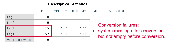
Only flag3 and flag4 contain some conversion failures. We can visually inspect what's the problem by moving these cases to the top of our dataset.
sort cases by flag3 (d).
*Some values flagged with 'a'.
sort cases by flag4 (d).
*Some values flagged with 'a' through 'e'.
Result
Remove Illegal Characters, Copy and Convert
Some values are flagged with letters “a” through “e”, which is why they fail to convert. We'll now fix the problem. First, we close our data without saving and reopen it. We then rerun our previous syntax but remove these letters before the conversion.
Syntax
*Copy all stringvars.
string c1 to c4 (a7).
recode s1 to s4 (else = copy) into c1 to c4.
*Remove 'a' from s3.
compute s3 = replace(s3,'a','').
*Remove 'a' through 'e' from s4.
do repeat #char = 'a' 'b' 'c' 'd' 'e'.
compute s4 = replace(s4,#char,'').
end repeat.
*Try and convert variable again.
alter type s1 to s3 (f1) s4 (f6.3).
*Flag conversion failures again.
do repeat #conv = s1 to s4 / #ori = c1 to c4 / #flags = flag1 to flag4.
if(sysmis(#conv) and #ori <> '') #flags = 1.
end repeat.
*Inspect if conversion succeeded.
descriptives flag1 to flag4.
*N = 0 for all flag variables so we're done.
*Delete copied and flag variables.
delete variables c1 to flag4.
Result
All flag variables contain only (system) missings. This means that we no longer have any conversion failures; all variables have been correctly converted. We can now delete all copy and flag variables, save our data and move on.
Thanks for reading!
Quick Overview SPSS Operators and Functions
The table below presents a quick overview of functions and operators in SPSS, sorted by type (numeric, string, ...). Details and examples for some lesser known functions are covered below the table.
| TYPE | Function | DESCRIPTION | EXAMPLE |
|---|---|---|---|
| Comparison | = (or EQ) | Equal to | if(var01 = 0) var02 = 1. |
| Comparison | <> (or NE) | Not equal to | if(var01 <> 0) var02 = 1. |
| Comparison | < (or LT) | Less than | if(var01 < 0) var02 = 1. |
| Comparison | <= (or LE) | At most | if(var01 <= 0) var02 = 1. |
| Comparison | > (or GT) | Greater than | if(var01 > 0) var02 = 1. |
| Comparison | >= (or GE) | At least | if(var01 >= 0) var02 = 1. |
| Comparison | RANGE | Within range | if(range(score,0,20) grp01 = 1. |
| Comparison | ANY | First value among second, third, ... values? | if(any(nation,1,3,5)) flag01 = 1. |
| Logical | & (or AND) | All arguments true? | if(sex = 0 & score >= 100) grp01 = 1. |
| Logical | | (or OR) | At least 1 argument true? | if(sex = 0 | score <= 90) grp01 = 1. |
| Logical | NOT | Argument not true | select if(not(missing(score))). |
| Numeric | + | Addition | compute sum01 = var01 + var02. |
| Numeric | - | Subtraction | compute dif01 = var01 - var02. |
| Numeric | * | Multiplication | compute revenue = sales * price. |
| Numeric | / | Division | compute avg01 = sum01 / trials. |
| Numeric | ** | Exponentiation | compute square01 = var01**2. |
| Numeric | SQRT | Square root | compute root01 = sqrt(var01). |
| Numeric | RND | Round | compute score = rnd(reactime). |
| Numeric | MOD | Modulo Function | compute cntr = mod(id,4). |
| Numeric | TRUNC | Truncate | compute score = trunc(reactime). |
| Numeric | ABS | Absolute value | compute abs01 = abs(score). |
| Numeric | EXP | Exponential Function | compute escore = exp(score). |
| Numeric | LN | Natural logarithm | compute lnscore = ln(score). |
| Statistical | MIN | Minimum over variables | compute min01 = min(var01 to var10). |
| Statistical | MAX | Maximum over variables | compute max01 = max(var01 to var10). |
| Statistical | SUM | Sum over variables | compute total = sum(var01 to var10). |
| Statistical | MEAN | Mean over variables | compute m01 = mean(var01 to var10). |
| Statistical | MEDIAN | Median over variables | compute me01 = median(var01 to var10). |
| Statistical | VARIANCE | Variance over variables | compute vnc01 = variance(var01 to var10). |
| Statistical | SD | Standard deviation over variables | compute sd01 = sd(var01 to var10). |
| Missing | MISSING | System or user missing | select if(missing(score)). |
| Missing | SYSMIS | System missing | select if(not(sysmis(score))). |
| Missing | NMISS | Count missing values over variables | compute mis01 = nmiss(v01 to v10). |
| Missing | NVALID | Count valid values over variables | compute val01 = nvalid(v01 to v10). |
| String | LOWER | Convert to lowercase | compute sku = lower(sku). |
| String | UPCASE | Convert to uppercase | compute sku = upcase(sku). |
| String | CHAR.LENGTH | Number of characters in string | compute len01 = char.length(firstname). |
| String | CHAR.INDEX | Position of first occurrence of substring | compute pos01 = char.index('banana','a'). |
| String | CHAR.RINDEX | Position of last occurrence of substring | compute pos02 = char.rindex('banana','a'). |
| String | CHAR.SUBSTR | Extract substring | compute firstchar = char.substr(name,1,1). |
| String | CONCAT | Concatenate strings | compute name = concat(fname,' ',lname). |
| String | REPLACE | Replace substring | compute str01 = replace('dog','g','t'). |
| String | RTRIM | Right trim string | compute str02 = rtrim(str02). |
| String | LTRIM | Left trim string | compute str03 = ltrim(str03). |
| Date | DATE.DMY | Convert day, month, year into date | compute mydate = date.dmy(31,1,2024). |
| Date | DATEDIFF | Compute difference between dates in chosen time units | compute age = datediff(datevar02,datevar01,'years'). |
| Date | DATESUM | Add time units to date | compute followup = datesum(datevar01,100,'days'). |
| Date | XDATE | Extract date component from date | compute byear = xdate.year(bdate). |
| Time | TIME.HMS | Convert hours, minutes, seconds into time | compute time01 = time.hms(17,45,12). |
| Distribution | CDF | Cumulative probability distribution or density Function | compute pvalue = cdf.normal(-1.96,0,1). |
| Distribution | IDF | Inverse probability distribution or density Function | compute zvalue95 = idf.normal(.025,0,1). |
| Distribution | Probability distribution or density Function | compute prob = pdf.binom(0,10,.5). | |
| Distribution | RV | Draw (pseudo) random numbers from specified probability distribution or density Function | compute rand01 = rv.uniform(0,1). |
| Other | LAG | Retrieve value from previous case | compute prev = lag(varname). |
| Other | NUMBER | Convert string to number | compute nvar = number(svar,f3). |
| Other | STRING | Convert number to string | compute svar = string(nvar,f3). |
| Other | VALUELABEL | Set value labels as string values | compute svar = valuelabel(nvar). |
SPSS ANY Function Example
In SPSS, ANY evaluates if the first value is among the second, third, ... values. So for example, let's say we want to know if the completion day was a Monday, Wednesday or a Friday? We could use if(cday = 2 or cday = 4 or cday = 6) flag01 = 1. However, a nice shorthand here is if(any(cday,2,4,6)) flag01 = 1. The screenshot below shows the result when run on spss-functions.sav.
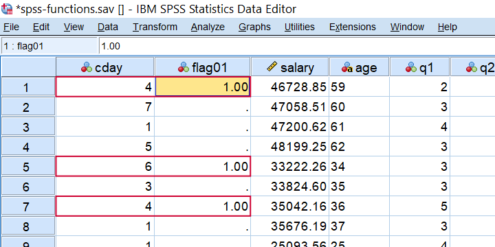 Result of IF(ANY(CDAY,2,4,6)) FLAG01 = 1.
As a second example, let's flag all cases who scored at least one 1 among the last 5 variables. This is often done with COUNT and then RECODE but a shorter option is if(any(1,q1 to q5)) flag02 = 1. which checks if the value 1 is among variables q1 to q5.
SPSS RND Function Example
In SPSS, you can round a value x to some constant c which is 1 by default. Like so,
RND(123456.789) = 123457RND(123456.789,10) = 123460 andRND(123456.789,.1) = 123456.8.
So for rounding salaries to dollars, you could use compute salary = rnd(salary). Alternatively, use compute salary = rnd(salary,.01). for rounding to dollar cents. For rounding salaries to thousands of dollars, use compute salary = rnd(salary,1000). as shown below when run on spss-functions.sav.
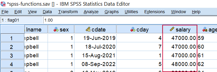 Result of COMPUTE SALARY = RND(SALARY,1000).
SPSS MOD Function Example
In SPSS, MOD is short for the modulo function where MOD(X,Y) returns the remainder of X after subtracting Y from it as many times as possible. This comes in handy for creating a trial counter if each respondent has the same number of trials as in compute trial = mod(($casenum - 1),4) + 1. When run on spss-functions.sav, the result is shown below.
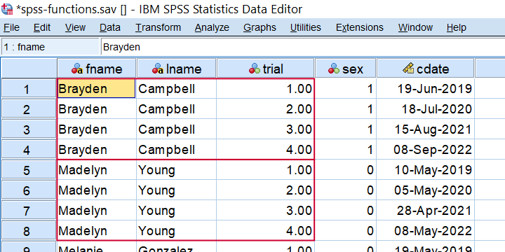 Trial counter created by COMPUTE TRIAL = MOD(($CASENUM - 1),4) + 1.
SPSS TRUNC Function Example
In SPSS, you can truncate (“round down”) a value x to some constant c which is 1 by default. Like so,
- TRUNC(123456.789) = 123456
- TRUNC(123456.789,10) = 123450 and
- TRUNC(123456.789,.1) = 123456.7.
TRUNC comes in handy for creating a respondent identifier if each respondent has the same number of trials as in compute respid = trunc(($casenum - 1) / 4) + 1. The result is shown below when run on spss-functions.sav.
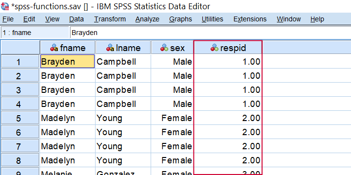 Result from COMPUTE RESPID = TRUNC(($CASENUM - 1) / 4) + 1.
SPSS MEAN Function Example
In SPSS, MEAN is pretty straightforward but there's 2 things you should know: first off, if there's any missing values, then
$$mean = \frac{sum(valid\;values)}{number\;of\;valid\;values}$$
This is important because the number of valid values may differ over respondents.
Second, you can restrict MEAN to a minimal number of valid values, k, by using MEAN.k(...). So for spss-functions.sav, compute m01 = mean.5(q1 to q5). only computes mean scores over cases not having any missing values over these 5 variables as shown below.
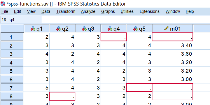 Result from COMPUTE M01 = MEAN.5(Q1 TO Q5).
SPSS SD Function Example
In SPSS, SD computes the standard deviation over variables. It has the same properties discussed for MEAN. SD comes in handy for detecting “straightliners” (respondents giving the same answer to all or most questions). Like so, compute sd01 = sd(q1 to q5). quickly does the job for spss-functions.sav.
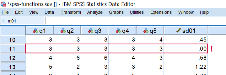 Detecting straightliners with COMPUTE SD01 = SD(Q1 TO Q5).
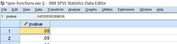
SPSS CDF Function Example
CDF is short for cumulative (probability) density (or distribution) function: it returns $$P(X \le x)$$,
given some probability density function. For example, assuming that z follows a standard normal distribution,
what's the 2-tailed p-value for z = -2.0?
We can find this out by running
compute pvalue = 2 * cdf.normal(-2,0,1).
as shown below.
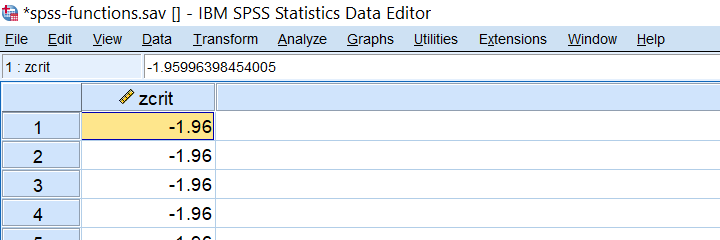
SPSS IDF Function Example
IDF is short for inverse (probability) density (or distribution) function: it returns a critical value for some chosen probability, given a density function. Note that this is exactly what we do when computing confidence intervals. For example: which z-value has a cumulative probability of .025? Well, we can compute this by compute zcrit = idf.normal(.025,0,1). as shown below.
SPSS NUMBER Function Example
In SPSS, NUMBER converts a string variable into a (new) numeric one. With regard to spss-functions.sav, compute nage = number(age,f2). creates a numeric age variable based on the string variable containing age.
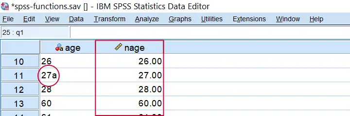 Result from COMPUTE NAGE = NUMBER(AGE,F2). Note the illegal character for case 11.
Importantly, choosing the f2 format results in SPSS ignoring all but the first 2 characters. If we choose f3 instead as in compute nage = number(age,f3). then SPSS throws the following warning:
>An invalid numeric field has been found. The result has been set to the
>system-missing value.
>Command line: 117 Current case: 11 Current splitfile group: 1
>Field contents: '27a'
This is because the age for case 11 contains an illegal character, resulting in a system missing value. Sadly, when converting this variable with ALTER TYPE,
this value simply disappears from your data
without any warning or error.
In our opinion, this really is a major stupidity in SPSS and very tricky indeed.
SPSS VALUELABEL Function Example
The VALUELABEL function sets the value labels for some variable as the values for some string variable. The syntax below illustrates how it's done for spss-functions.sav.
string sday(a10).
*SET VALUE LABELS FOR CDAY AS VALUES.
compute sday = valuelabel(cday).
execute.
Result
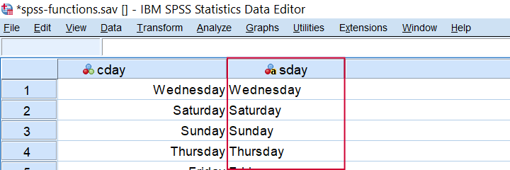 Result from COMPUTE SDAY = VALUELABEL(CDAY).
Final Notes
Now honestly, our overview of SPSS operators and functions is not 100% comprehensive. I did leave out some examples that are so rare that covering them mostly just clutters up the table without helping anybody.
If you've any questions or remarks, please leave a comment below. And other than that:
thanks for reading!
SPSS 27 – Quick Review
On 19 June 2020, SPSS version 27 was released. Although it has some useful new features, most of these have been poorly implemented. This review quickly walks you through the main improvements and their limitations.
- Cohen’s D - Effect Size for T-Tests
- SPSS 27 - Power & Sample Size Calculations
- APA Frequency Tables
- Python Version 2.x Deprecated
- SPSS’ Search Function
- Bootstrapping Included in SPSS Base
Cohen’s D - Effect Size for T-Tests
Cohen’s D is the main effect size measure for all 3 t-tests:
- the independent samples t-test,
- the paired samples t-test and
- the one sample t-test.
SPSS users have been complaining for ages about Cohen’s D being absent from SPSS. However, SPSS 27 finally includes it as shown below.
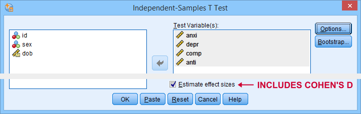
The only way to obtain Cohen’s D is selecting “Estimate effect sizes”. Sadly, this results in a separate table that contains way more output than we typically want.

So why does this suck?
- The APA reporting guidelines ask for a single table containing the significance tests and Cohen’s D. Meeting this standard requires copy-pasting results from separate SPSS tables manually -never a good idea.
- The excessive output confuses users. I'll bet a monthly salary that the “Standardizer” instead of the “Point estimate” will be reported as Cohen’s D on a pretty regular basis.
So what's the right way to go?
The right way to go is found in JASP. The figure below shows how it implements Cohen’s D.
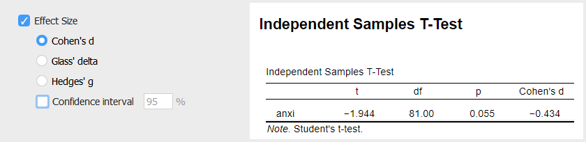
So what makes this better than the SPSS implementation? Well,
- JASP allows us to choose which effect size measure it reports;
- we can choose which confidence interval it reports -optionally none;
- JASP reports all results in a single table;
- Cohen’s D is called “Cohen’s d” rather than “Point estimate”.
Power & Sample Size Calculations - The Basics
Before we turn to power calculations in SPSS 27, let's first revisit some minimal basics.
Computing power or required sample sizes involves 4 statistics:
- α -often 0.05- is the probability of making a Type I error: rejecting some null hypothesis if it's actually true;
- (1 - β) or power -often 0.80- is the probability of rejecting some null hypothesis given some exact alternative hypothesis, often expressed as an effect size;
- effect size is a standardized number that summarizes to what extent some null hypothesis is not true -either in a sample or a population;
- sample size is the number of independent observations involved in some significance test.
We can compute each of these 4 statistics if we know the other 3. In practice, we usually don't know these but we can still make educated guesses. These result in different scenarios that can easily be calculated. This is mostly done for
- computing required sample sizes for different effect sizes given a chosen α and (1 - β);
- computing power for different sample sizes given a chosen α and (1 - β).
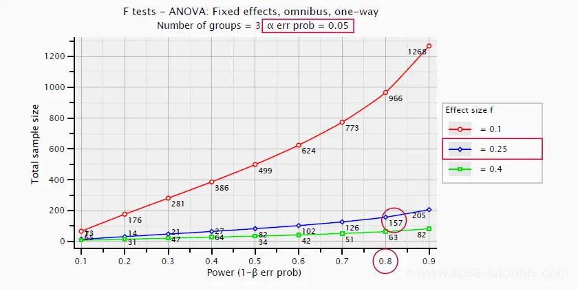
So let's say we want compare 3 different medicines. We're planning a 3-group ANOVA at α = 0.05 and we want (1 - β) = 0.80. We guess that the effect size, Cohen’s f = 0.25 (medium).
Given this scenario, we should use a total sample size of N = 157 participants as shown below.
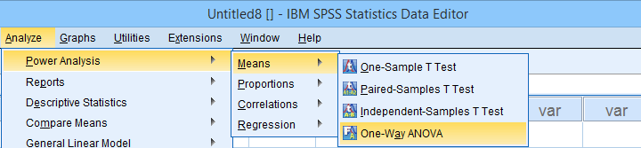
SPSS 27 - Power & Sample Size Calculations
Now let's say we want to know the required sample size for a 4-way ANOVA. We'll first open the power analysis dialog as shown below.
In the dialog that opens (below),
 we'll select “Estimate sample size”
 we'll enter the power or (1 - β) we desire;
 we'll enter the alpha level or α at which we're planning to test.
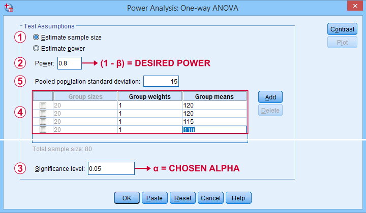
Our sample size calculation requires just one more number: the expected effect size. But for some very stupid reason,
we can't enter any effect size in this dialog.
Instead, SPSS will compute it for us if we enter
 all expected means and
 the expected Pooled population standard deviation.
The problem is that you probably won't have a clue what to enter here: since we run this analysis before collecting any data, we can't look up the required statistics.
So how does effect size make that situation any better? Well, first off, effect size is a single number as opposed to the separate numbers required by the dialog. And because it's a single number, we can consult simple rules of thumb such as
- f = 0.10 indicates a small effect;
- f = 0.25 indicates a medium effect;
- f = 0.40 indicates a large effect.
Such estimated effect sizes can be directly entered in G*Power as shown below. It does not require 4 (unknown) means and an (unknown) standard deviation. However, you can optionally compute effect size from these numbers and proceed from there.
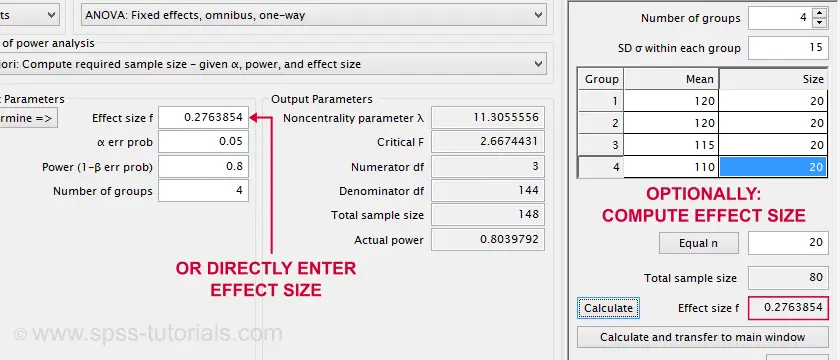
Note that the GPower dialog also contains the main output: we should collect data on a total sample size of N = 148 independent observations.
Next, we reran this analysis in SPSS 27. The output is shown below.
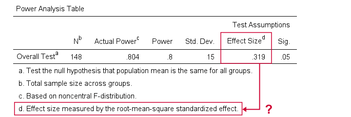 Sample size calculation output example from SPSS 27
Fortunately, the SPSS and GPower conclusions are almost identical. But for some weird reason, SPSS reports the “root-mean-square standardized effect” as its effect size measure.
Common effect size measures for ANOVA are
- η2 or (partial) eta-squared;
- ω2 or omega-squared;
- Cohen’s f.
The aforementioned output includes none of those. Reversely, (partial) eta-squared is the only effect size measure we obtain if we actually run the ANOVA in SPSS.
We could now look into the plots from SPSS power analysis. Or we could discuss why chi-square tests are completely absent. But let's not waste time.
SPSS power analysis is pathetic.
Use GPower instead.
APA Frequency Tables
Basic frequency distributions are the most fundamental tables in all of statistics. Sadly, those in SPSS are confusing to users and don't comply with APA guidelines. That's why we published Creating APA Style Frequency Tables in SPSS some years ago.
SPSS 27 finally offers similar tables. For creating them, navigate to
![]()
![]() and follow the steps below.
and follow the steps below.
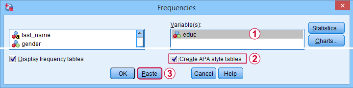
These steps result in the syntax below.
FREQUENCIES VARIABLES=educ jtype
/ORDER=ANALYSIS.
OUTPUT MODIFY
/REPORT PRINTREPORT=NO
/SELECT TABLES
/IF COMMANDS=["Frequencies(LAST)"] SUBTYPES="Frequencies"
/TABLECELLS SELECT=[VALIDPERCENT] APPLYTO=COLUMN HIDE=YES
/TABLECELLS SELECT=[CUMULATIVEPERCENT] APPLYTO=COLUMN HIDE=YES
/TABLECELLS SELECT=[TOTAL] SELECTCONDITION=PARENT(VALID) APPLYTO=ROW HIDE=YES
/TABLECELLS SELECT=[TOTAL] SELECTCONDITION=PARENT(MISSING) APPLYTO=ROW HIDE=YES
/TABLECELLS SELECT=[VALID] APPLYTO=ROWHEADER UNGROUP=YES
/TABLECELLS SELECT=[PERCENT] SELECTDIMENSION=COLUMNS FORMAT="PCT" APPLYTO=COLUMN
/TABLECELLS SELECT=[COUNT] APPLYTO=COLUMNHEADER REPLACE="N"
/TABLECELLS SELECT=[PERCENT] APPLYTO=COLUMNHEADER REPLACE="%".
A standard FREQUENCIES command creates the tables and OUTPUT MODIFY then adjusts them. This may work but it requires 14 lines of syntax. Our approach -combining COMPUTE and MEANS- requires only 3 as shown below.
compute constant = 0.
means constant by educ jtype
/cells count npct.
*Optionally, set nicer column headers.
output modify
/select tables
/if commands = ["means(last)"]
/tablecells select = [percent] applyto = columnheader replace = '%'.
So why does SPSS 27 need 14 lines of syntax if we really need only 3? Surely, it must create much better output, right? Well... No. Let's carefully compare the results from both approaches.
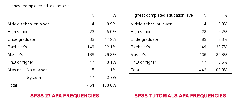
- The SPSS 27 approach always includes user missing values -whether you want it or not. The only way to exclude them is using some type of FILTER. Note that you probably need different filters for different tables -very tedious indeed.
- By default, our approach excludes user missing values. However, you can choose to include them by adding /MISSING INCLUDE to the MEANS command. This also works fine if you run many tables in one go.
- SPSS 27 always includes system missing values.
- Our approach never includes system missing values. However, you can include them if you RECODE them into user missing values, possibly preceded by TEMPORARY.
In short, we feel the SPSS 27 approach is worse on all accounts than what we proposed in Creating APA Style Frequency Tables in SPSS some years ago.
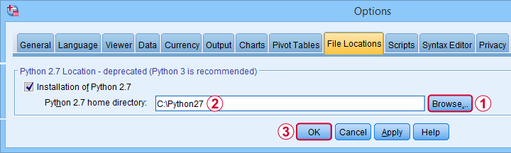
Python Version 2.x Deprecated
By default, SPSS 27 no longer supports Python 2.x. This makes sense because the Python developers themselves deprecated version 2 around April 2020.
For us, it's bad new because we're still using tons of scripts and tools in Python 2. We're well aware that we should rewrite those in Python 3 but we don't have the time for it now. Fortunately,
you can still use Python 2 in SPSS 27.
First, simply install Python 2.7 on your system. Next, navigate to
![]() and select the tab. Finally, Follow the steps shown below.
and select the tab. Finally, Follow the steps shown below.
After completing these steps, you can use Python 2 in SPSS 27. One issue, however, is that SPSS throws a >Warning # 8501 Command name: begin program each time you run anything in Python 2. If you run a large number of Python 2 blocks, this becomes seriously annoying.
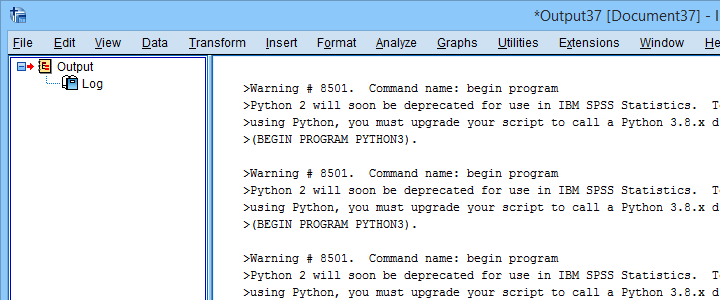
You can prevent these warnings by running SET ERRORS NONE. prior to running any Python blocks. After you're done with those, make sure you switch the errors back on by running SET ERRORS LISTING. This is a pretty poor solution, though. We tried to prevent only the aforementioned Warning # 8501 but we didn't find any way to get it done.
Last but not least, deprecating Python 2 in favor of Python 3 probably causes compatibility issues: SPSS versions 13-23 can only be used with Python 2, not Python 3. So for these SPSS versions, we must build our tools in Python 2. Sadly, those tools won't work “out of the box” anymore with SPSS 27.
SPSS’ Search Function
SPSS 27 comes with a search function that supposedly finds “help topics, dialogs and case studies”. Our very first attempt was searching for “kruskal” for finding information on the Kruskal-Wallis test. Although SPSS obviously includes this test, the search dialog came up with zero results.
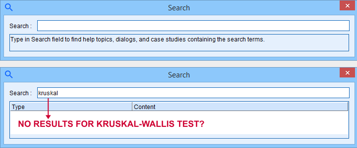
We didn't explore the search function any further.
Bootstrapping Included in SPSS Base
Very basically, bootstrapping estimates standard errors and sampling distributions. It does so by simulating a simple random sampling procedure by resampling observations from a sample. Like so, it doesn't rely on the usual statistical assumptions such as normally distributed variables.
Traditionally, you could bootstrap statistics in SPSS by using
- a macro (this is how the PROCESS dialog bootstraps its results);
- an SPSS Python script or;
- the Bootstrap option: an SPSS add-on module which requires an additional license.
SPSS 27 no longer requires the aforementioned additional license: it includes the Bootstrap option by default. This is a nice little bonus for SPSS users upgrading from previous versions.
Conclusions
The good news about SPSS 27 is that it implements some useful new features that users actually need. Some examples covered in this review are
- Cohen’s D for t-tests;
- APA frequency tables and;
- power and sample size calculations.
The bad news, however, is that these features have been poorly implemented. They look and feel as if they were developed solely by statisticians and programmers without consulting any
- SPSS users;
- UX professionals;
- competing software -most notably JASP and GPower.
The end result looks like a poor attempt at reinventing the wheel.
So that's what we think. So what about you? Did you try SPSS 27 and what do you think about it? Let us know by throwing a quick comment below. We love to hear from you.
Thanks for reading!
Opening Excel Files in SPSS
- Open Excel File with Values in SPSS
- Apply Variable Labels from Excel
- Apply Value Labels from Excel
- Open Excel Files with Strings in SPSS
- Converting String Variables from Excel
Excel files containing social sciences data mostly come in 2 basic types:
- files containing data values (1, 2, ...) and variable names (v01, v02, ...) and separate sheets on what the data represents as shown in course-evaluation-values.xlsx;
- files containg answer categories (“Good”, “Bad”, ...) and question descriptions (“How did you find...”) as in course-evaluation-labels.xlsx.
Just opening either file in SPSS is simple. However, preparing the data for analyses may be challenging. This tutorial quickly walks you through.
Open Excel File with Values in SPSS
Let's first fix course-evaluation-values.xlsx, partly shown below.
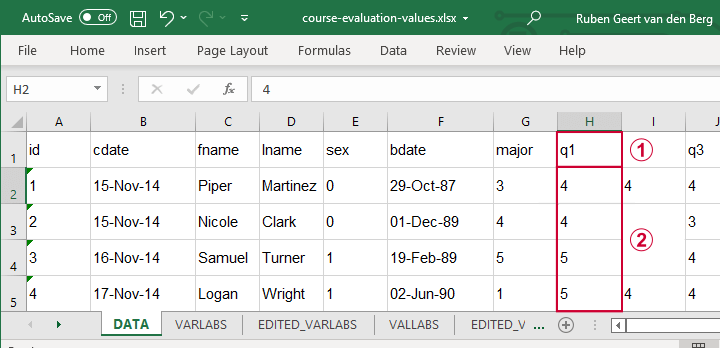
 The data sheet has short variable names whose descriptions are in another sheet, VARLABS (short for “variable labels”);
 Answer categories are represented by numbers whose descriptions are in VALLABS (short for “value labels”).
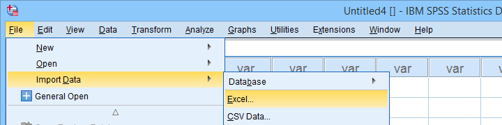
Let's first simply open our actual data sheet in SPSS by navigating to
![]()
![]() as shown below.
as shown below.
Next up, fill out the dialogs as shown below. Tip: you can also open these dialogs if you drag & drop an Excel file into an SPSS Data Editor window.
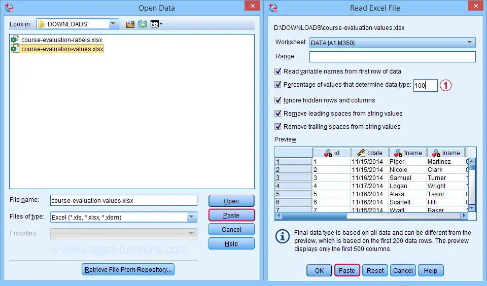
By default, SPSS converts Excel columns to numeric variables if at least 95% of their values are numbers. Other values are converted to system missing values without telling you which or how many values have disappeared. This is very risky but we can prevent this by setting it to 100.
Completing these steps results in the SPSS syntax shown below.
GET DATA
/TYPE=XLSX
/FILE='D:\data\course-evaluation-values.xlsx'
/SHEET=name 'DATA'
/CELLRANGE=FULL
/READNAMES=ON
/LEADINGSPACES IGNORE=YES
/TRAILINGSPACES IGNORE=YES
/DATATYPEMIN PERCENTAGE=100.0
/HIDDEN IGNORE=YES.
Result
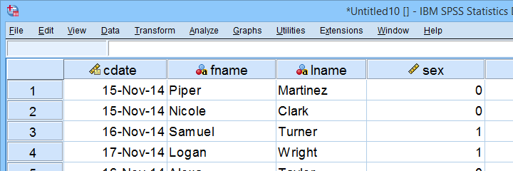
As shown, our actual data are now in SPSS. However, we still need to add their labels from the other Excel sheets. Let's start off with variable labels.
Apply Variable Labels from Excel
A quick and easy way for setting variable labels is creating SPSS syntax with Excel formulas: we basically add single quotes around each label and precede it with the variable name as shown below.
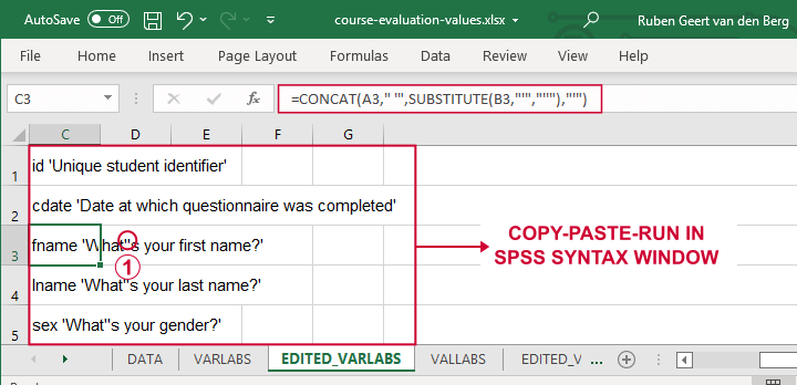
If we use single quotes around labels, we need to replace single quotes within labels by 2 single quotes.
Finally, we simply copy-paste these cells into a syntax window, precede it with VARIABLE LABELS and end the final line with a period. The syntax below shows the first couple of lines thus created.
variable labels
id 'Unique student identifier'
cdate 'Date at which questionnaire was completed'.
Apply Value Labels from Excel
We'll now set value labels with the same basic trick. The Excel formulas are a bit harder this time but still pretty doable.
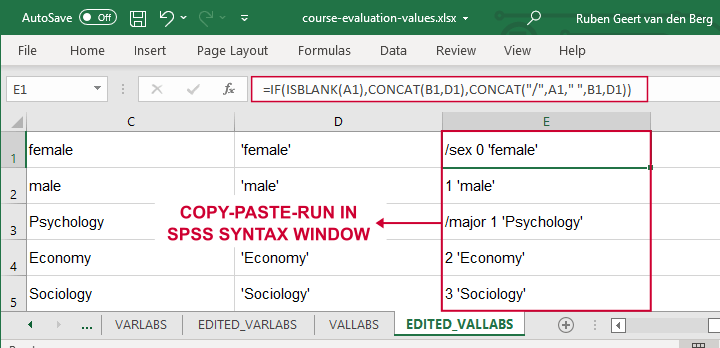
Let's copy-paste column E into an SPSS syntax window and add VALUE LABELS and a period to it. The syntax below shows the first couple of lines.
value labels
/sex 0 'female'
1 'male'
/major 1 'Psychology'
2 'Economy'
3 'Sociology'
4 'Anthropology'
5 'Other'.
After running these lines, we're pretty much done with this file. Quick note: if you need to convert many Excel files, you could automate this process with a simple Python script.
Open Excel Files with Strings in SPSS
Let's now convert course-evaluation-labels.xlsx, partly shown below.
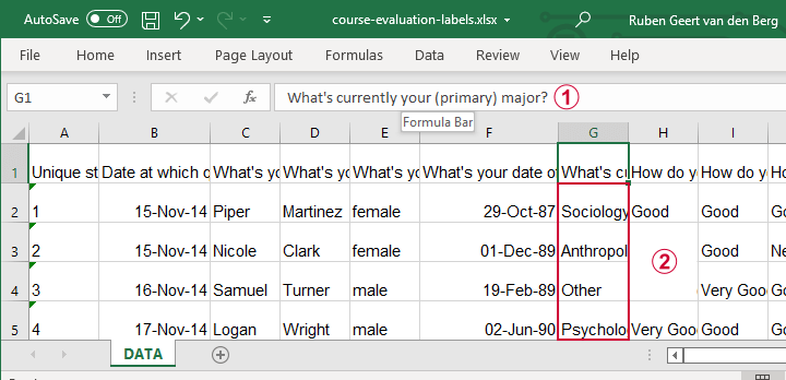
Note that the Excel column headers are full question descriptions;
the Excel cells contain the actual answer categories.
Let's first open this Excel sheet in SPSS. We'll do so with the exact same steps as in Open Excel File with Values in SPSS, resulting in the syntax below.
GET DATA
/TYPE=XLSX
/FILE='d:/data/course-evaluation-labels.xlsx'
/SHEET=name 'DATA'
/CELLRANGE=FULL
/READNAMES=ON
/LEADINGSPACES IGNORE=YES
/TRAILINGSPACES IGNORE=YES
/DATATYPEMIN PERCENTAGE=100.0
/HIDDEN IGNORE=YES.
Result
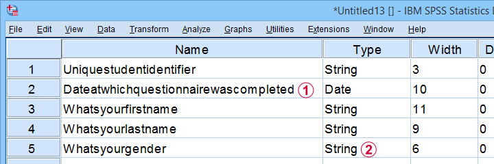
This Excel sheet results in huge variable names in SPSS;
most Excel columns have become string variables in SPSS.
Let's now fix both issues.
Shortening Variable Names
I strongly recommend using short variable names. You can set these with RENAME VARIABLES (ALL = V01 TO V13). Before doing so, make sure all variables have decent variable labels. If some are empty, I often set their variable names as labels. That's usually all information we have from the Excel column headers.
A simple little Python script for doing so is shown below.
begin program python3.
import spss
spssSyn = ''
for i in range(spss.GetVariableCount()):
varlab = spss.GetVariableLabel(i)
if not varlab:
varnam = spss.GetVariableName(i)
if not spssSyn:
spssSyn = 'VARIABLE LABELS'
spssSyn += "\n%(varnam)s '%(varnam)s'"%locals()
if spssSyn:
print(spssSyn)
spss.Submit(spssSyn + '.')
end program.
Converting String Variables from Excel
So how to convert our string variables to numeric ones? This depends on what's in these variables:
- for quantitative string variables containing numbers, try ALTER TYPE;
- for nominal answer categories, try AUTORECODE;
- for ordinal answer categories, use RECODE or try AUTORECODE and then adjust their order.
For example, the syntax below converts “id” to numeric.
alter type v01 (f8).
*CHECK FOR SYSTEM MISSING VALUES AFTER CONVERSION.
descriptives v01.
*SET COLUMN WIDTH SOMEWHAT WIDER FOR V01.
variable width v01 (6).
*AND SO ON...
Just as the Excel-SPSS conversion, ALTER TYPE may result in values disappearing without any warning or error as explained in SPSS ALTER TYPE Reporting Wrong Values?
If your converted variable doesn't have any system missing values, then this problem has not occurred. However, if you do see some system missing values, you'd better find out why these occur before proceeding.
Converting Ordinal String Variables
The easy way to convert ordinal string variables to numeric ones is to
- AUTORECODE them and
- adjust the order of the answer categories.
We thoroughly covered this method SPSS - Recode with Value Labels Tool (example II). Do look it up and try it. It may save you a lot of time and effort.
If you're somehow not able to use this method, a basic RECODE does the job too as shown below.
recode v08 to v13
('Very bad' = 1)
('Bad' = 2)
('Neutral' = 3)
('Good' = 4)
('Very Good' = 5)
into n08 to n13.
*SET VALUE LABELS.
value labels n08 to n13
1 'Very bad'
2 'Bad'
3 'Neutral'
4 'Good'
5 'Very Good'.
*SET VARIABLE LABELS.
variable labels
n08 'How do you rate this course?'
n09 'How do you rate the teacher of this course?'
n10 'How do you rate the lectures of this course?'
n11 'How do you rate the assignments of this course?'
n12 'How do you rate the learning resources (such as syllabi and handouts) that were issued by us?'
n13 'How do you rate the learning resources (such as books) that were not issued by us?'.
Keep in mind that writing such syntax sure sucks.
So that's about it for today. If you've any questions or remarks, throw me a comment below.
Thanks for reading!
Normalizing Variable Transformations – 6 Simple Options
- Overview Transformations
- Normalizing - What and Why?
- Normalizing Negative/Zero Values
- Test Data
- Descriptives after Transformations
- Conclusion
Overview Transformations
| TRANSFORMATION | USE IF | LIMITATIONS | SPSS EXAMPLES |
|---|---|---|---|
| Square/Cube Root | Variable shows positive skewness Residuals show positive heteroscedasticity Variable contains frequency counts | Square root only applies to positive values | compute newvar = sqrt(oldvar). compute newvar = oldvar**(1/3). |
| Logarithmic | Distribution is positively skewed | Ln and log10 only apply to positive values | compute newvar = ln(oldvar). compute newvar = lg10(oldvar). |
| Power | Distribution is negatively skewed | (None) | compute newvar = oldvar**3. |
| Inverse | Variable has platykurtic distribution | Can't handle zeroes | compute newvar = 1 / oldvar. |
| Hyperbolic Arcsine | Distribution is positively skewed | (None) | compute newvar = ln(oldvar + sqrt(oldvar**2 + 1)). |
| Arcsine | Variable contains proportions | Can't handle absolute values > 1 | compute newvar = arsin(oldvar). |
Normalizing - What and Why?
“Normalizing” means transforming a variable in order to
make it more normally distributed.
Many statistical procedures require a normality assumption: variables must be normally distributed in some population. Some options for evaluating if this holds are
- inspecting histograms;
- inspecting if skewness and (excess) kurtosis are close to zero;
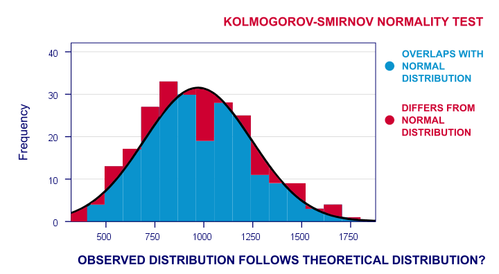
- running a Shapiro-Wilk test and/or a Kolmogorov-Smirnov test.
For reasonable sample sizes (say, N ≥ 25), violating the normality assumption is often no problem: due to the central limit theorem, many statistical tests still produce accurate results in this case. So why would you normalize any variables in the first place? First off, some statistics -notably means, standard deviations and correlations- have been argued to be technically correct but still somewhat misleading for highly non-normal variables.
Second, we also encounter normalizing transformations in multiple regression analysis for
- meeting the assumption of normally distributed regression residuals;
- reducing heteroscedasticity and;
- reducing curvilinearity between the dependent variable and one or many predictors.
Normalizing Negative/Zero Values
Some transformations in our overview don't apply to negative and/or zero values. If such values are present in your data, you've 2 main options:
- transform only non-negative and/or non-zero values;
- add a constant to all values such that their minimum is 0, 1 or some other positive value.
The first option may result in many missing data points and may thus seriously bias your results. Alternatively, adding a constant that adjusts a variable's minimum to 1 is done with
$$Pos_x = Var_x - Min_x + 1$$
This may look like a nice solution but keep in mind that a minimum of 1 is completely arbitrary: you could just as well choose, 0.1, 10, 25 or any other positive number. And that's a real problem because the constant you choose may affect the shape of a variable's distribution after some normalizing transformation. This inevitably induces some arbitrariness into the normalized variables that you'll eventually analyze and report.
Test Data
We tried out all transformations in our overview on 2 variables with N = 1,000:
- var01 has strong negative skewness and runs from -1,000 to +1,000;
- var02 has strong positive skewness and also runs from -1,000 to +1,000;
These data are available from this Googlesheet (read-only), partly shown below.
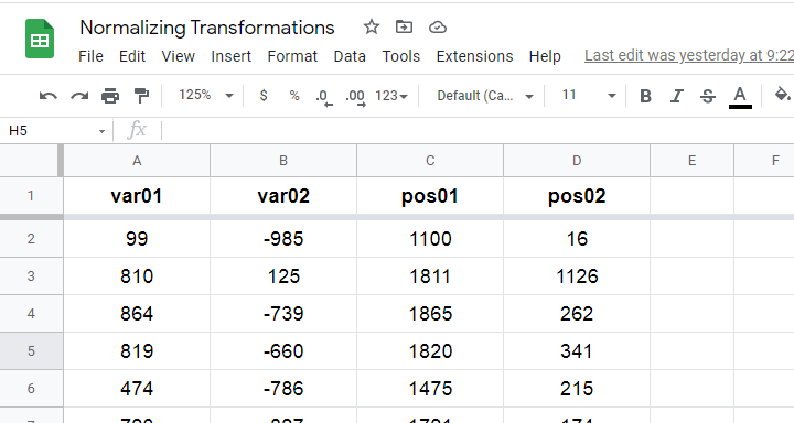
SPSS users may download the exact same data as normalizing-transformations.sav.
Since some transformations don't apply to negative and/or zero values, we “positified” both variables: we added a constant to them such that their minima were both 1, resulting in pos01 and pos02.
Although some transformations could be applied to the original variables, the “normalizing” effects looked very disappointing. We therefore decided to limit this discussion to only our positified variables.
Square/Cube Root Transformation
A cube root transformation did a great job in normalizing our positively skewed variable as shown below.
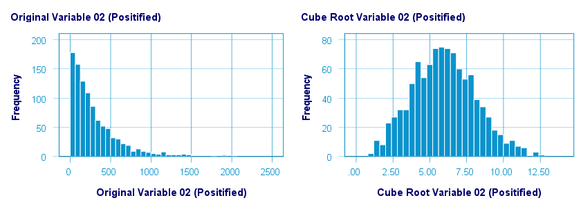
The scatterplot below shows the original versus transformed values.
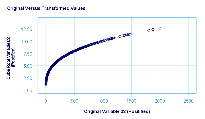
SPSS refuses to compute cube roots for negative numbers. The syntax below, however, includes a simple workaround for this problem.
compute curt01 = pos01**(1/3).
compute curt02 = pos02**(1/3).
*NOTE: IF VARIABLE MAY CONTAIN NEGATIVE VALUES, USE.
*if(pos01 >= 0) curt01 = pos01**(1/3).
*if(pos01 < 0) curt01 = -abs(pos01)**(1/3).
*HISTOGRAMS.
frequencies curt01 curt02
/format notable
/histogram.
*SCATTERPLOTS.
graph/scatter pos01 with curt01.
graph/scatter pos02 with curt02.
Logarithmic Transformation
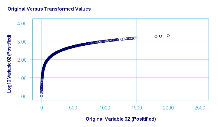
A base 10 logarithmic transformation did a decent job in normalizing var02 but not var01. Some results are shown below.
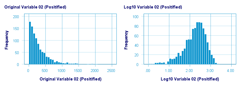
The scatterplot below visualizes the original versus transformed values.
SPSS users can replicate these results from the syntax below.
compute log01 = lg10(pos01).
compute log02 = lg10(pos02).
*HISTOGRAMS.
frequencies log01 log02
/format notable
/histogram.
*SCATTERPLOTS.
graph/scatter pos01 with log01.
graph/scatter pos02 with log02.
Power Transformation
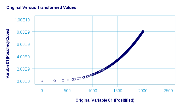
A third power (or cube) transformation was one of the few transformations that had some normalizing effect on our left skewed variable as shown below.
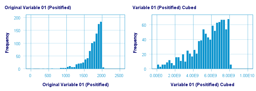
The scatterplot below shows the original versus transformed values for this transformation.
These results can be replicated from the syntax below.
compute cub01 = pos01**3.
compute cub02 = pos02**3.
*HISTOGRAMS.
frequencies cub01 cub02
/format notable
/histogram.
*SCATTERS.
graph/scatter pos01 with cub01.
graph/scatter pos02 with cub02.
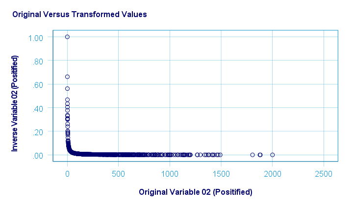
Inverse Transformation
The inverse transformation did a disastrous job with regard to normalizing both variables. The histograms below visualize the distribution for pos02 before and after the transformation.
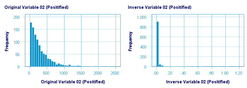
The scatterplot below shows the original versus transformed values. The reason for the extreme pattern in this chart is setting an arbitrary minimum of 1 for this variable as discussed under normalizing negative values.
SPSS users can use the syntax below for replicating these results.
compute inv01 = 1 / pos01.
compute inv02 = 1 / pos02.
*NOTE: IF VARIABLE MAY CONTAIN ZEROES, USE.
*if(pos01 <> 0) inv01 = 1 / pos01.
*HISTOGRAMS.
frequencies inv01 inv02
/format notable
/histogram.
*SCATTERPLOTS.
graph/scatter pos01 with inv01.
graph/scatter pos02 with inv02.
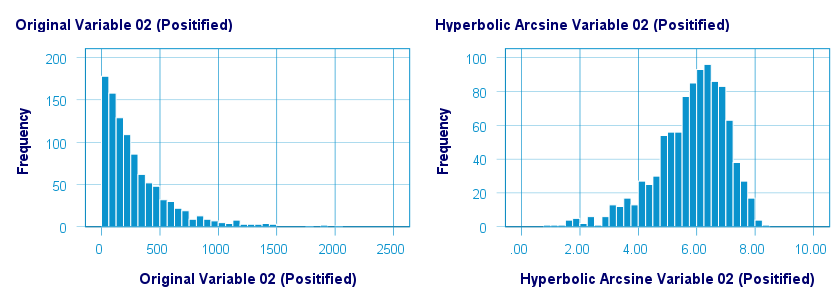
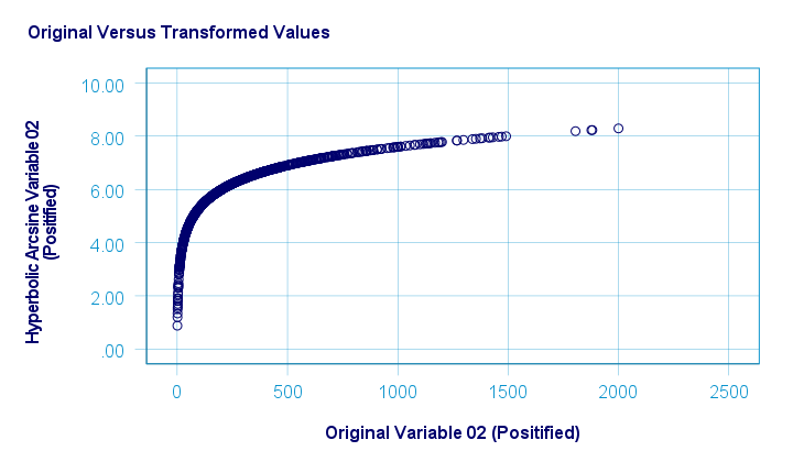
Hyperbolic Arcsine Transformation
As shown below, the hyperbolic arcsine transformation had a reasonably normalizing effect on var02 but not var01.
The scatterplot below plots the original versus transformed values.
In Excel and Googlesheets, the hyperbolic arcsine is computed from =ASINH(...) There's no such function in SPSS but a simple workaround is using
$$Asinh_x = ln(Var_x + \sqrt{Var_x^2 + 1})$$
The syntax below does just that.
compute asinh01 = ln(pos01 + sqrt(pos01**2 + 1)).
compute asinh02 = ln(pos02 + sqrt(pos02**2 + 1)).
*HISTOGRAMS.
frequencies asinh01 asinh02
/format notable
/histogram.
*SCATTERS.
graph/scatter pos01 with asinh01.
graph/scatter pos02 with asinh02.
Arcsine Transformation
Before applying the arcsine transformation, we first rescaled both variables to a range of [-1, +1]. After doing so, the arcsine transformation had a slightly normalizing effect on both variables. The figure below shows the result for var01.
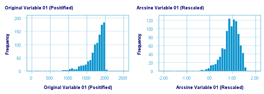
The original versus transformed values are visualized in the scatterplot below.
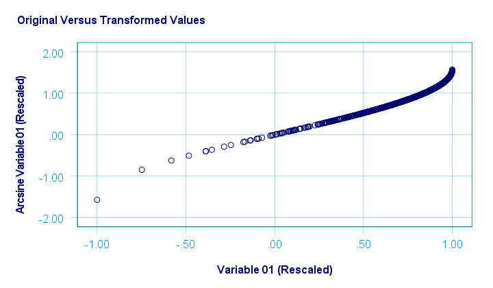
The rescaling of both variables as well as the actual transformation were done with the SPSS syntax below.
aggregate outfile * mode addvariables
/min01 min02 = min(var01 var02)
/max01 max02 = max(var01 var02).
*RESCALE VARIABLES TO [-1, +1] .
compute trans01 = (var01 - min01)/(max01 - min01)*2 - 1.
compute trans02 = (var02 - min01)/(max01 - min01)*2 - 1.
*ARCSINE TRANSFORMATION.
compute asin01 = arsin(trans01).
compute asin02 = arsin(trans02).
*HISTOGRAMS.
frequencies asin01 asin02
/format notable
/histogram.
*SCATTERS.
graph/scatter trans01 with asin01.
graph/scatter trans02 with asin02.
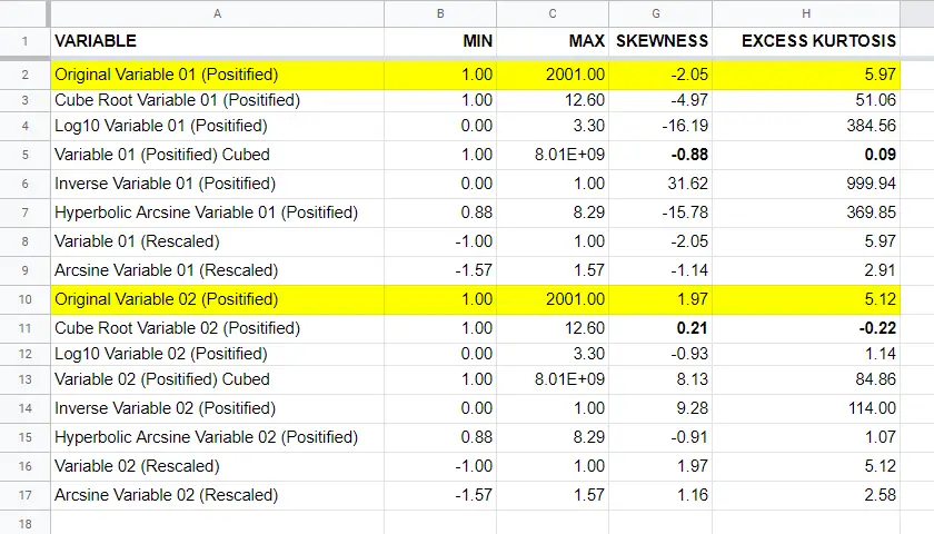
Descriptives after Transformations
The figure below summarizes some basic descriptive statistics for our original variables before and after all transformations. The entire table is available from this Googlesheet (read-only).
Conclusion
If we only judge by the skewness and kurtosis after each transformation, then for our 2 test variables
- the third power transformation had the strongest normalizing effect on our left skewed variable and
- the cube root transformation worked best for our right skewed variable.
I should add that none of the transformations did a really good job for our left skewed variable, though.
Obviously, these conclusions are based on only 2 test variables. To what extent they generalize to a wider range of data is unclear. But at least we've some idea now.
If you've any remarks or suggestions, please throw us a quick comment below.
Thanks for reading.
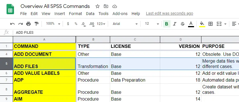
Quick Overview All SPSS Commands
A quick, simple and complete overview of all SPSS commands is presented in this Googlesheet, partly shown below.
For each command, our overview includes
Let's quickly walk through each of these components.
SPSS Command Types
SPSS commands come in 3 basic types:
- transformations are commands that are not immediately executed. Most transformations (IF, RECODE, COMPUTE, COUNT) are used for creating new variables. Transformations can be used in loops (DO REPEAT or LOOP) and/or conditionally (DO IF).
- procedures are commands that inspect all cases in the active dataset. Procedures are mostly used for data analysis such as running charts, tables and statistical tests. Procedures also cause transformations to be executed.
- other commands are neither transformations, nor procedures.
Required License
SPSS has a modular structure: you always need a base license, which you can expand with one or more licenses for additional modules.Very confusingly, modules are sometimes referred to as “options” in some documentation. Perhaps they will be referred to as “SPSS Apps” at some point in the future... The most useful modules are
- Advanced Statistics (repeated measures ANOVA, MANOVA and loglinear analysis);
- Regression (logistic regression);
- Missing Values (analysis of missing values and multiple imputation).
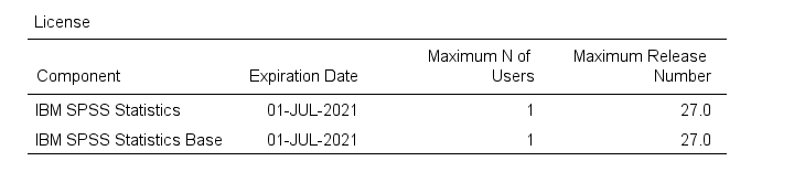
You can only use features from modules for which you're licensed. If you're not sure, running show license. prints a quick overview in your output window as shown below.
SPSS Versions
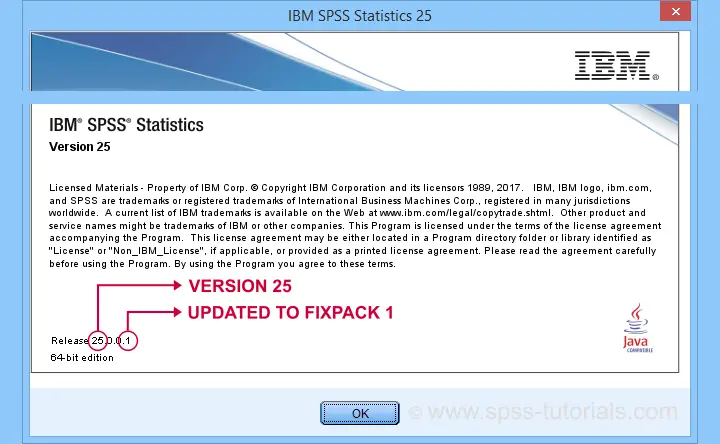
SPSS presents a new version roughly once a year. The latest version is SPSS 27, launched in May 2020. So which commands can you (not) use if you're on an older version? Look it up straight away in our overview.Quick note: commands that were introduced before SPSS 12 have been listed as version 12. We couldn't find any older documentation and we don't expect anybody to use such ancient versions anymore. Correct me if I'm wrong...
Not sure which SPSS version you're on?
Just run
show license.
and you'll find out. Alternatively, consulting
![]() also tells you which patches (“Fixpacks”) you've installed as shown below.I think this latter method is available only on Windows systems. I'm not sure about that as I avoid Apple like the plague.
also tells you which patches (“Fixpacks”) you've installed as shown below.I think this latter method is available only on Windows systems. I'm not sure about that as I avoid Apple like the plague.
Right. I hope you find my overview helpful. If you've any remarks or questions, please throw me a comments below.
Thanks for reading!
How to Find & Exclude Outliers in SPSS?
- Method I - Histograms
- Excluding Outliers from Data
- Method II - Boxplots
- Method III - Z-Scores (with Reporting)
- Method III - Z-Scores (without Reporting)
Summary
Outliers are basically values that fall outside of a normal range for some variable. But what's a “normal range”? This is subjective and may depend on substantive knowledge and prior research. Alternatively, there's some rules of thumb as well. These are less subjective but don't always result in better decisions as we're about to see.
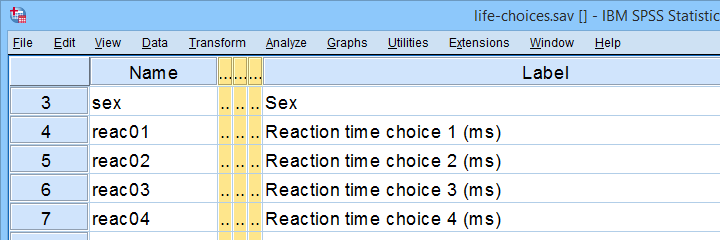
In any case: we usually want to exclude outliers from data analysis. So how to do so in SPSS? We'll walk you through 3 methods, using life-choices.sav, partly shown below.
 In this tutorial, we'll find outliers for these reaction time variables.
During this tutorial, we'll focus exclusively on reac01 to reac05, the reaction times in milliseconds for 5 choice trials offered to the respondents.
Method I - Histograms
Let's first try to identify outliers by running some quick histograms over our 5 reaction time variables. Doing so from SPSS’ menu is discussed in Creating Histograms in SPSS. A faster option, though, is running the syntax below.
frequencies reac01 to reac05
/histogram.
Result
Let's take a good look at the first of our 5 histograms shown below.
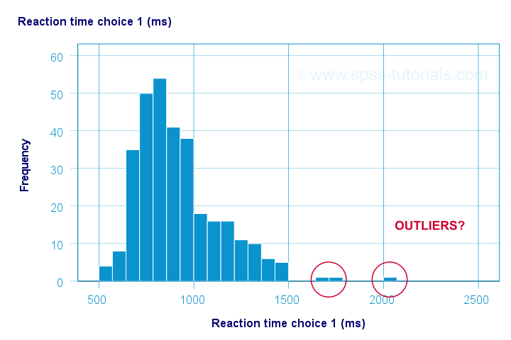
The “normal range” for this variable seems to run from 500 through 1500 ms. It seems that 3 scores lie outside this range. So are these outliers? Honestly, different analysts will make different decisions here. Personally, I'd settle for only excluding the score ≥ 2000 ms. So what's the right way to do so? And what about the other variables?
Excluding Outliers from Data
The right way to exclude outliers from data analysis is to specify them as user missing values. So for reaction time 1 (reac01), running missing values reac01 (2000 thru hi). excludes reaction times of 2000 ms and higher from all data analyses and editing. So what about the other 4 variables?
The histograms for reac02 and reac03 don't show any outliers.
For reac04, we see some low outliers as well as a high outlier. We can find which values these are in the bottom and top of its frequency distribution as shown below.
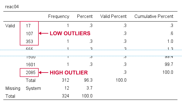 If we see any outliers in a histogram, we may look up the exact values in the corresponding frequency table.
We can exclude all of these outliers in one go by running missing values reac04 (lo thru 400,2085). By the way: “lo thru 400” means the lowest value in this variable (its minimum) through 400 ms.
For reac05, we see several low and high outliers. The obvious thing to do seems to run something like missing values reac05 (lo thru 400,2000 thru hi). But sadly, this only triggers the following error:
>There are too many values specified.
>The limit is three individual values or
>one value and one range of values.
>Execution of this command stops.
The problem here is that
you can't specify a low and a high
range of missing values in SPSS.
Since this is what you typically need to do, this is one of the biggest stupidities still found in SPSS today. A workaround for this problem is to
- RECODE the entire low range into some huge value such as 999999999;
- add the original values to a value label for this value;
- specify only a high range of missing values that includes 999999999.
The syntax below does just that and reruns our histograms to check if all outliers have indeed been correctly excluded.
recode reac05 (lo thru 400 = 999999999).
*Add value label to 999999999.
add value labels reac05 999999999 '(Recoded from 95 / 113 / 397 ms)'.
*Set range of high missing values.
missing values reac05 (2000 thru hi).
*Rerun frequency tables after excluding outliers.
frequencies reac01 to reac05
/histogram.
Result
First off, note that none of our 5 histograms show any outliers anymore; they're now excluded from all data analysis and editing. Also note the bottom of the frequency table for reac05 shown below.
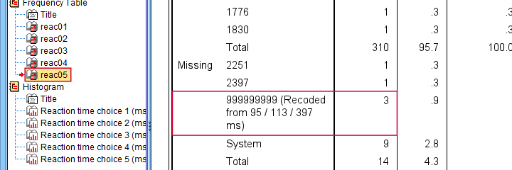 Low outliers after recoding and labelling are listed under Missing.
Even though we had to recode some values, we can still report precisely which outliers we excluded for this variable due to our value label.
Before proceeding to boxplots, I'd like to mention 2 worst practices for excluding outliers:
- removing outliers by changing them into system missing values. After doing so, we no longer know which outliers we excluded. Also, we're clueless why values are system missing as they don't have any value labels.
- removing entire cases -often respondents- because they have 1(+) outliers. Such cases typically have mostly “normal” data values that we can use just fine for analyzing other (sets of) variables.
Sadly, supervisors sometimes force their students to take this road anyway. If so, SELECT IF permanently removes entire cases from your data.
Method II - Boxplots
If you ran the previous examples, you need to close and reopen life-choices.sav before proceeding with our second method.
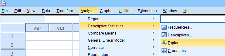
We'll create a boxplot as discussed in Creating Boxplots in SPSS - Quick Guide: we first navigate to
![]()
![]() as shown below.
as shown below.
Next, we'll fill in the dialogs as shown below.
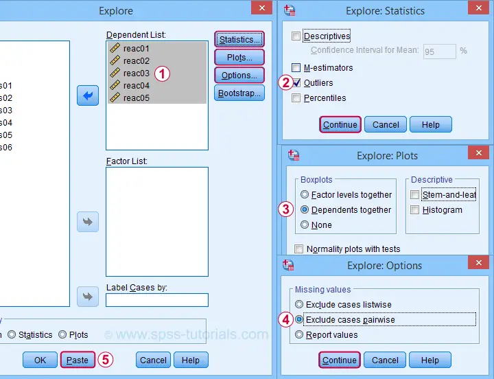
Completing these steps results in the syntax below. Let's run it.
EXAMINE VARIABLES=reac01 reac02 reac03 reac04 reac05
/PLOT BOXPLOT
/COMPARE VARIABLES
/STATISTICS EXTREME
/MISSING PAIRWISE
/NOTOTAL.
Result
Quick note: if you're not sure about interpreting boxplots, read up on Boxplots - Beginners Tutorial first.
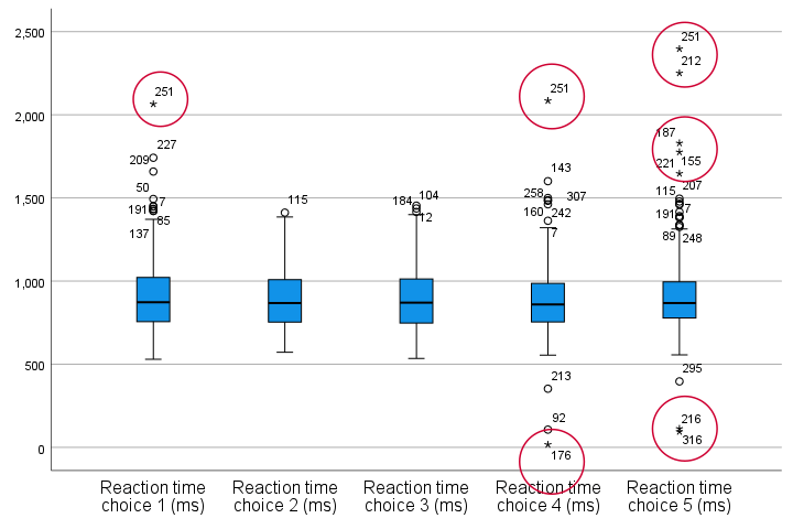
Our boxplot indicates some potential outliers for all 5 variables. But let's just ignore these and exclude only the extreme values that are observed for reac01, reac04 and reac05.
So, precisely which values should we exclude? We find them in the Extreme Values table. I like to copy-paste this into Excel. Now we can easily boldface all values that are extreme values according to our boxplot.
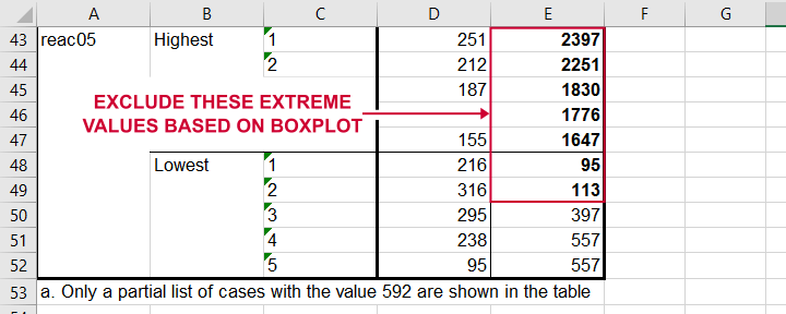 Copy-pasting the Extreme Values table into Excel allows you to easily boldface the exact outliers that we'll exclude.
Finally, we set these extreme values as user missing values with the syntax below. For a step-by-step explanation of this routine, look up Excluding Outliers from Data.
recode reac05 (lo thru 113 = 999999999).
*Label new value with original values.
add value labels reac05 999999999 '(Recoded from 95 / 113 ms)'.
*Set (ranges of) missing values for reac01, reac04 and reac05.
missing values
reac01 (2065)
reac04 (17,2085)
reac05 (1647 thru hi).
*Rerun boxplot and check if all extreme values are gone.
EXAMINE VARIABLES=reac01 reac02 reac03 reac04 reac05
/PLOT BOXPLOT
/COMPARE VARIABLES
/STATISTICS EXTREME
/MISSING PAIRWISE
/NOTOTAL.
Method III - Z-Scores (with Reporting)
A common approach to excluding outliers is to look up which values correspond to high z-scores. Again, there's different rules of thumb which z-scores should be considered outliers. Today, we settle for |z| ≥ 3.29 indicates an outlier. The basic idea here is that if a variable is perfectly normally distributed, then only 0.1% of its values will fall outside this range.
So what's the best way to do this in SPSS? Well, the first 2 steps are super simple:
- we add z-scores for all relevant variables to our data and
- see if their minima or maxima meet |z| ≥ 3.29.
Funnily, both steps are best done with a simple DESCRIPTIVES command as shown below.
descriptives reac01 to reac05
/save.
*Check min and max for z-scores.
descriptives zreac01 to zreac05.
Result
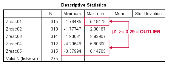 Minima and maxima for our newly computed z-scores.
Basic conclusions from this table are that
- reac01 has at least 1 high outlier;
- reac02 and reac03 don't have any outliers;
- reac04 and reac05 both have at least 1 low and 1 high outlier.
But which original values correspond to these high absolute z-scores? For each variable, we can run 2 simple steps:
- FILTER away cases having |z| < 3.29 (all non outliers);
- run a frequency table -now containing only outliers- on the original variable.
The syntax below does just that but uses TEMPORARY and SELECT IF for filtering out non outliers.
temporary.
select if(abs(zreac01) >= 3.29).
frequencies reac01.
temporary.
select if(abs(zreac04) >= 3.29).
frequencies reac04.
temporary.
select if(abs(zreac05) >= 3.29).
frequencies reac05.
*Save output because tables needed for reporting which outliers are excluded.
output save outfile = 'outlier-tables-01.spv'.
Result
 Finding outliers by filtering out all non outliers based on their z-scores.
Note that each frequency table only contains a handful of outliers for which |z| ≥ 3.29. We'll now exclude these values from all data analyses and editing with the syntax below. For a detailed explanation of these steps, see Excluding Outliers from Data.
recode reac04 (lo thru 107 = 999999999).
recode reac05 (lo thru 113 = 999999999).
*Label new values with original values.
add value labels reac04 999999999 '(Recoded from 17 / 107 ms)'.
add value labels reac05 999999999 '(Recoded from 95 / 113 ms)'.
*Set (ranges of) missing values for reac01, reac04 and reac05.
missing values
reac01 (1659 thru hi)
reac04 (1601 thru hi )
reac05 (1776 thru hi).
*Check if all outliers are indeed user missing values now.
temporary.
select if(abs(zreac01) >= 3.29).
frequencies reac01.
temporary.
select if(abs(zreac04) >= 3.29).
frequencies reac04.
temporary.
select if(abs(zreac05) >= 3.29).
frequencies reac05.
Method III - Z-Scores (without Reporting)
We can greatly speed up the z-score approach we just discussed but this comes at a price: we won't be able to report precisely which outliers we excluded. If that's ok with you, the syntax below almost fully automates the job.
descriptives reac01 to reac05
/save.
*Recode original values into 999999999 if z-score >= 3.29.
do repeat #ori = reac01 to reac05 / #z = zreac01 to zreac05.
if(abs(#z) >= 3.29) #ori = 999999999.
end repeat print.
*Add value labels.
add value labels reac01 to reac05 999999999 '(Excluded because |z| >= 3.29)'.
*Set missing values.
missing values reac01 to reac05 (999999999).
*Check how many outliers were exluded.
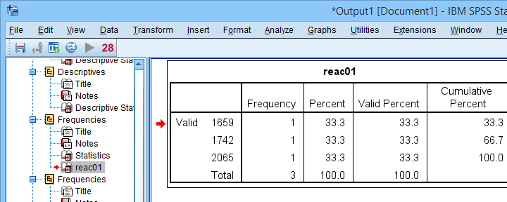
frequencies reac01 to reac05.
Result
The frequency table below tells us that 4 outliers having |z| ≥ 3.29 were excluded for reac04.
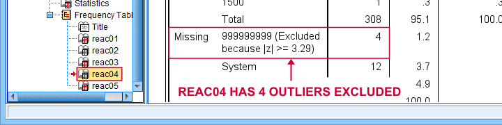 Under Missing we see the number of excluded outliers but not the exact values.
Sadly, we're no longer able to tell precisely which original values these correspond to.
Final Notes
Thus far, I deliberately avoided the discussion precisely which values should be considered outliers for our data. I feel that simply making a decision and being fully explicit about it is more constructive than endless debate.
I therefore blindly followed some rules of thumb for the boxplot and z-score approaches. As I warned earlier, these don't always result in good decisions: for the data at hand, reaction times below some 500 ms can't be taken seriously. However, the rules of thumb don't always exclude these.
As for most of data analysis, using common sense is usually a better idea...
Thanks for reading!
SPSS – Missing Values for String Variables
- Setting Missing Values for String Variables
- Missing String Values and MEANS
- Missing String Values and CROSSTABS
- Missing String Values and COMPUTE
- Workarounds for Bugs
Can you set missing values for string variables in SPSS? Short answer: yes. Sadly, however, this doesn't work as it should. This tutorial walks you through some problems and fixes.
Example Data
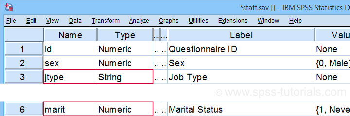
All examples in this tutorial use staff.sav, partly shown below. We'll run some basic operations on Job Type (a string variable) and Marital Status (a numeric variable) in parallel.
Let's first create basic some frequency distributions for both variables by running the syntax below.
frequencies marit jtype.
Result
Let's take a quick look at the frequency distribution for our string variable shown below.
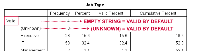
By default, all values in a string variable are valid (not missing), including an empty string value of zero characters.
Setting Missing Values for String Variables
Now, let's suppose we'd like to set the empty string value and (Unknown) as user missing values. Experienced SPSS users may think that running missing values jtype ('','(Unknown)'). should do the job. Sadly, SPSS simply responds with a rather puzzling warning:
>The missing value is specified more than once.
First off, this warning is nonsensical: we didn't specify any missing value more than once. And even if we did. So what?
Second, the warning doesn't tell us the real problem. We'll find it out if we run
missing values jtype ('(Unknown)').
This triggers the warning below, which tells us that our user missing string value is simply too long.
>The missing value exceeds 8 bytes.
>Execution of this command stops.
A quick workaround for this problem is to simply RECODE '(Unknown)' into something shorter such as 'NA' (short for ‘Not Available”). The syntax below does just that. It then sets user missing values for Job Type and reruns the frequency tables.
recode jtype ('(Unknown)' = 'NA').
*Set 2 user missing values for string variable.
missing values jtype ('','NA').
*Quick check.
frequencies marit jtype.
Result
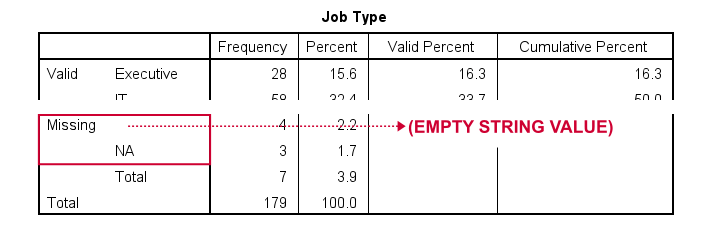
At this point, everything seems fine: both the empty string value and 'NA' are listed in the missing values section in our frequency table.
Missing String Values and MEANS
When running basic MEANS tables, user missing string values are treated as if they were valid. The syntax below demonstrates the problem:
means salary by marit jtype
/statistics anova.
Result
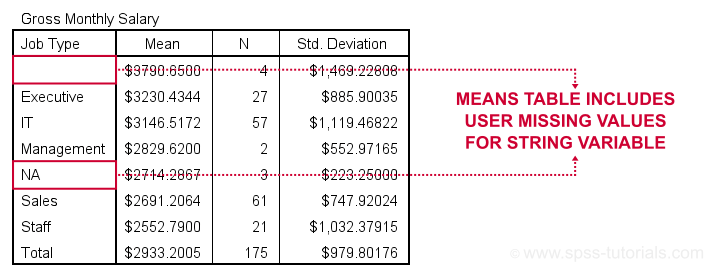
Note that user missing values are excluded in the first means table but included in the second means table. As this doesn't make sense and is not documented, I strongly suspect that this is a bug in SPSS.
Let's now try some CROSSTABS.
Missing String Values and CROSSTABS
We'll now run two basic contingency tables from the syntax below.
crosstabs marit jtype by sex.
Result
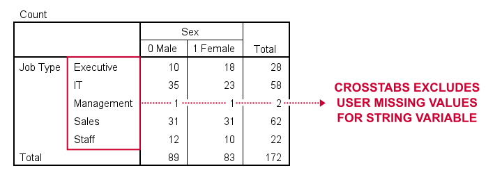
Basic conclusion: both tables fully exclude user missing values for our string and our numeric variables. This suggests that the aforementioned issue is restricted to MEANS. Unfortunately, however, there's more trouble...
Missing String Values and COMPUTE
A nice way to dichotomize variables is a single line COMPUTE as in
compute marr = (marit = 2).
In this syntax, (marit = 2) is a condition that may be false for some cases and true for others. SPSS returns 0 and 1 to represent false and true and hence creates a nice dummy variable.
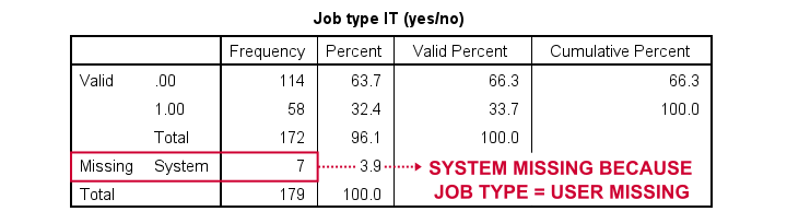
Now, if marit is (system or user) missing, SPSS doesn't know if the condition is true and hence returns a system missing value on our new variable. Sadly, this doesn't work for string variables as demonstrated below.
compute marr = (marit = 2).
variable labels marr 'Currently married (yes/no)'.
frequencies marr.
*Dichotomize string variable (incorrect result).
compute it = (jtype = 'IT').
variable labels it 'Job type IT (yes/no)'.
frequencies it.
A workaround for this problem is using IF. This shouldn't be necessary but it does circumvent the problem.
delete variables it.
*Dichotomize string variable (correct result).
if(not missing(jtype)) it = (jtype = 'IT').
variable labels it 'Job type IT (yes/no)'.
frequencies it.
Result
Workarounds for Bugs
The issues discussed in this tutorial are nasty; they may produce incorrect results that easily go unnoticed. A couple of ways to deal with them are the following:
- AUTORECODE string variables into numeric ones and proceed with these numeric counterparts.
- for creating tables and/or charts, exclude cases having string missing values with FILTER or even delete them altogether with SELECT IF.
- for creating new variables, IF and DO IF should suffice for most scenarios.
Right, I guess that should do regarding user missing string values. I hope you found my tutorial helpful. If you've any questions or comments, please throw us a comment below.
Thanks for reading!
SPSS 26 – Review of SPSS’ New Interface
SPSS 26 comes in both a new and the classic interface. We downloaded and tested the new interface. This review walks you through our main findings.
- SPSS 26 - Which “Subscription” Am I On?
- SPSS 26 - Data View & Variable View Tabs
- SPSS 26 - Menus & Dialogs
- SPSS 26 Output Tab - Tables & Charts
- SPSS 26 - The Analyze Catalog
- SPSS 26 - Conclusions
SPSS 26 - Which “Subscription” Am I On?
When downloading SPSS 26, we're offered both the new as well as the classic interface. Curiously, the IBM website mentions “SPSS Subscription” rather than “SPSS 26”.
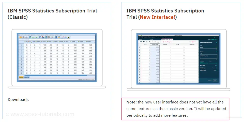
Before downloading it, we're already warned that the new interface “does not yet have all the same features” as the classic version. Well, ok. There's probably some tiny details they still need to work on. But they wouldn't launch a half-baked software package. Would they?
Anyway, we installed both versions and after doing so, our SPSS statistics directory looks like below.
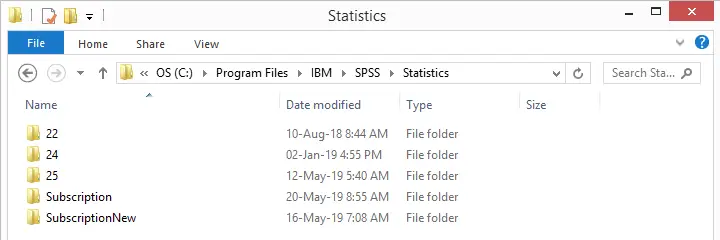
I was expecting a subfolder named 26 but instead I've Subscription and SubscriptionNew for the classic and new interfaces. It kinda makes me wonder
is this actually SPSS 26?
For SPSS 25 and older, this was always crystal clear: these versions mention their version number when starting or closing the program. In the middle of a session, navigating to
![]() shows the exact release such as 25.0.0.1. Alternatively, running the
show license. syntax would also do the trick.
shows the exact release such as 25.0.0.1. Alternatively, running the
show license. syntax would also do the trick.
In the new interface, none of those options come up with anything but “IBM SPSS Statistics”. However, when digging into the backend subfolder, we found stats.exe, the actual application. And when we hovered over the file, we saw this:
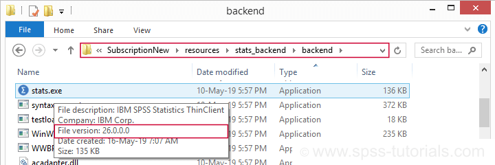
SPSS 26 indeed. But why do I even want to know my exact version number? Well,
- if something does not work in my SPSS version, I want to Google something like “SPSS 26 font size data editor”. If I can't add my version number to that, I'll get solutions for other SPSS versions that don't solve my problem.
- Second, if I want to help out my clients, their version numbers tell me what will (not) work for them.
- And -finally- the IBM license key center only offers me an authorization code for IBM SPSS Statistics Desktop 26. It does not mention any “Subscription” (see below).
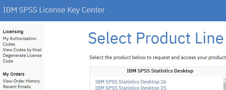
SPSS 26 - Data View & Variable View Tabs
Anway, we downloaded and installed the SPSS 26 with the new interface. After opening some data, we get the data view tab shown below.
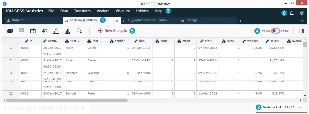
 The new interface is based on tabs rather than (data, syntax and output) windows. As we'll see in a minute, settings and dialogs also come as tabs.
 Variable view is below data view and slides up upon clicking it. We didn't discover any shortcut for doing so.
 The and menus are absent. I suppose they'll be added later. But for now, this really is a huge problem.
 The value/label switch does not toggle between values and value labels but -rather- between variable names and variable labels.
 An Analyze Catalog has been added.
 There's notifications and settings icons. However, these settings don't include the essential settings under
![]() in previous SPSS versions. These seem unavailable in the new interface.
in previous SPSS versions. These seem unavailable in the new interface.
SPSS 26 - Data View Issues
Even this very first exploration of the new interface resulted in some serious issues.
- First off, my laptop has a 1920 by 1080px screen resolution. As a result, the font sizes are way too small on my screen. Since there's no menu -the only way to set larger font sizes- this makes the new data view pretty useless for me.
- Second, it seems impossible to have multiple syntax tabs open simultaneously. Whenever I open another syntax file, the open syntax tab closes, asking me whether to save its contents.
- Third, my OUTPUT CLOSE command
triggers the error that it's no longer available. That sucks. I always start new projects with closing all open output and datasets. Some of my clients do the same. - Fourth, I like to toggle a lot between data view and variable view but -as mentioned- the Ctrl + t shortkey no longer works.
SPSS 26 - Variable View
In SPSS’ new interface, variable view is called “Variable List”. It's in the same tab as data view and slides up when clicked. Unfortunately, it no longer has the clear and simple structure known from previous SPSS versions.
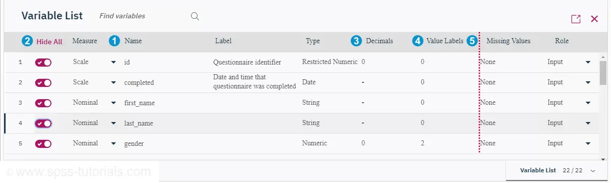
The order of variable properties has been altered with visibility and measurement levels before variable names.
The ability to hide variables is a welcome new feature. But what's the syntax for doing so? How to hide, say, v1 to v25 but not v26 to v50? That can't require 25 mouse clicks, right?
Width and columns have been removed. However, we'll get to those in a minute.
The value labels column is finally called “Value Labels” rather than “Values”. It now shows the number of labels defined for each variable.
Apart from the weird Serif fonts in Variable List, the alignment looks odd too: it seems some column headers are centered with their property values left aligned. Together with removing the classic grid, this doesn't contribute to a nice and clear interface.
We also noticed that clicking “Type” -which either refers to a variable type or format- opens up the dialog shown below.
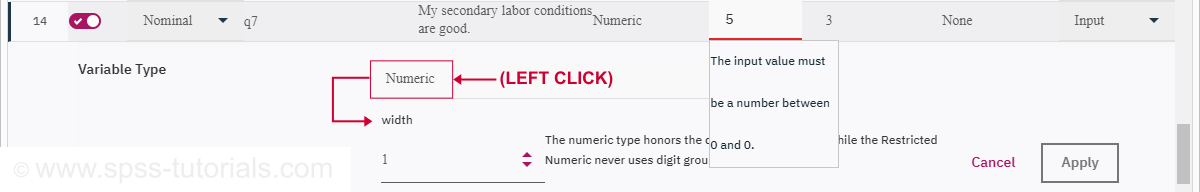 Variable type, width and format are shown when clicking “Type” in Variable List.
Note that a much better way to set formats and types are the FORMATS and ALTER TYPE commands: these can address many variables in one go and they are replicable.
SPSS 26 - Menus & Dialogs
For the most part, the new menus look like the old menus but incomplete and badly reorganized. For instance, let's take a look at as shown below.
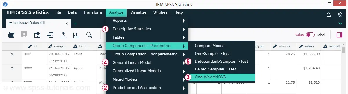
The most sought-after analyses in SPSS are
 The chi-square independence test -deeply hidden under Analyze
![]() Descriptive statistics
Descriptive statistics
![]() Crosstabs.
Crosstabs.
 Correlations, now hidden under Prediction and Association.
Regression, also under Prediction and Association.
 ANOVA, scattered over Group Comparison - Parametric and
  General Linear Model.
The independent samples t-test under Group Comparison - Parametric.
So why are the most popular analyses so hard to find? They're not meant to be literally “sought after”. These analyses should be listed at the top level of Analyze. Instead -however- Correlate and Regression have actually been removed from it.
SPSS 26 - Dialogs
The new dialogs look different from previous versions. Let's take a look at the Correlations dialog below.
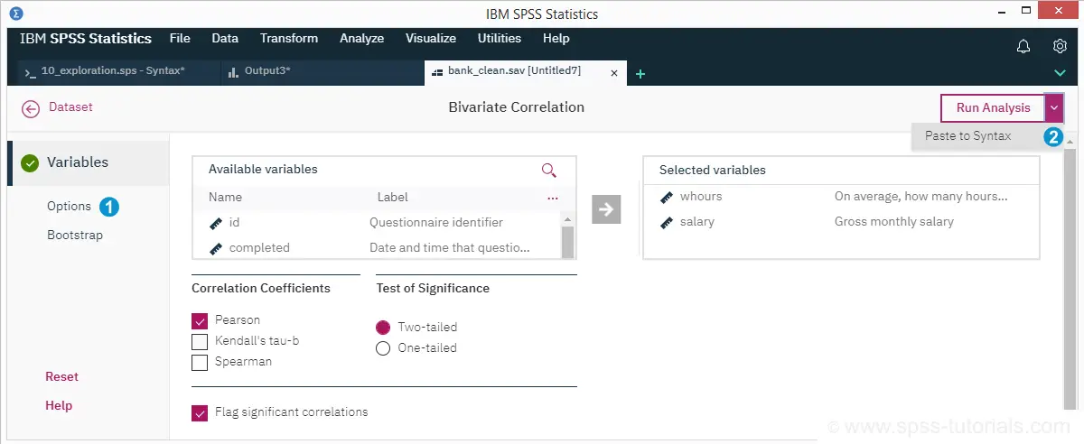
To our disappointment, the Options are still the same as in previous versions. And they are not good: regardless of what we need, we always get all significance levels in our output. Confidence intervals for correlations are still not available. We still can't choose whether we want any sample sizes included in our output table.
The classic functions such as Help and Ok are somewhat scattered over the dialog. Unfortunately, “Paste to syntax” is hidden under “Run Analysis” so this now takes 2 clicks instead of 1. The Alt based shortkeys and Esc no longer work either.
SPSS 26 Output Tab - Tables & Charts
After running our analysis, we're presented with the output tab shown below.
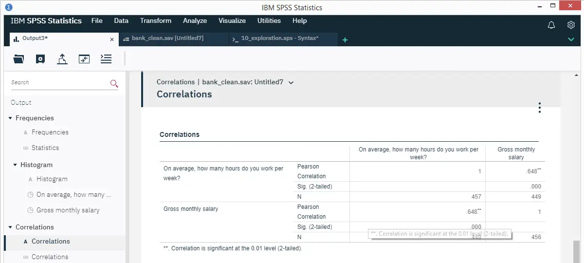
The output outline looks pretty nice and clean. However, when right-clicking an item, the OMS labels don't show up. For experienced users, this complicates batch editing tables with OUTPUT MODIFY.
The correlation table itself looks much better than previous SPSS versions as well. However, we stumbled upon some issues here too:
- Essential table editing functionality has disappeared. We managed to transpose the table but we can't rearrange its dimensions via Pivoting trays. Meeting APA standards for correlation tables is pretty much impossible from SPSS’ new interface.
- Tablelooks no longer seem to work, neither via the menu nor via syntax.
SPSS 26 - Charts
As shown below, charts still don't look too great in SPSS 26.
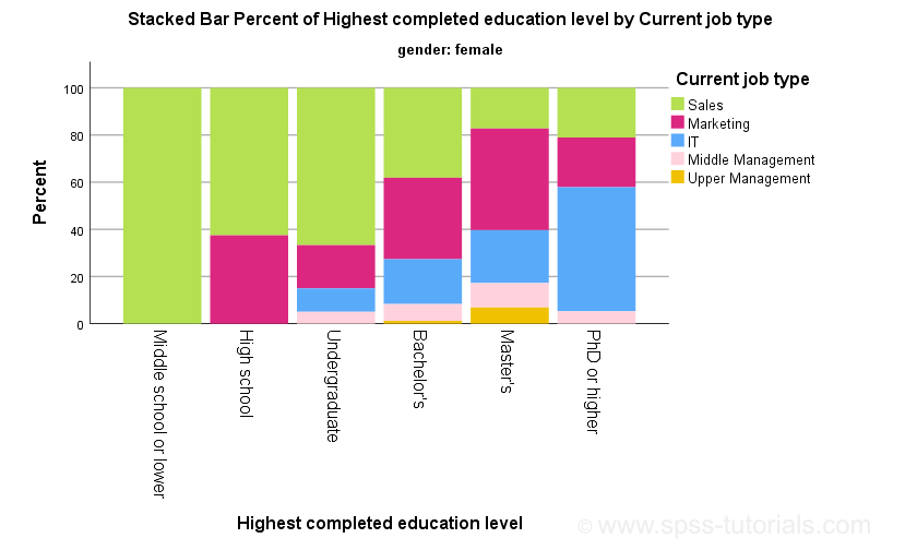
None of the issues discussed in New Charts in SPSS 25 - How Good Are They Really? have been resolved: still no percent sign on the y-axis. Still the wrong title. And so on.
More worrying, the SPSS 26 menu only includes the Chart builder. I sure hope the legacy dialogs will soon be added: they are much simpler and result in short and clean syntax that's copy-paste-editable.
SPSS 26 - The Analyze Catalog
Another new feature is the Analyze Catalog shown below. It's accessible from the Data View tab.
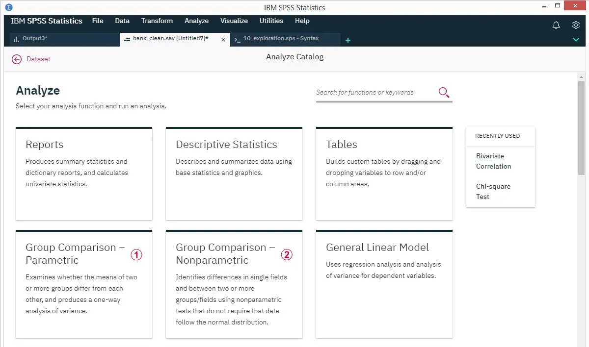
Sadly, the information here is incomplete and inaccurate.
For example, Group Comparison - Parametric doesn't mention any t-tests. Also, the one sample t-test and paired samples t-test don't compare “two or more groups”. The old description -“Compare Means”- did apply to all these tests.
Group Comparison - Nonparametric suggests that parametric tests require that “data follow the normal distribution”. This is wrong: the normality assumption is rarely required for reasonable sample sizes. This is why the Kolmogorov-Smirnov test is usually useless.
The way I see it is that
- SPSS users who don't know what to do need educational material optimized for educational purposes and
- SPSS users who know what to do need software optimized for production purposes.
A product that tries to combine these conflicting purposes will suck at both. This point could hardly be illustrated more convincingly than by the analyze catalog.
Anyway. One thing I do like about the analyze catalog is the search function. So I don't immediately see ANOVA anywhere in the menu but searching for it will surely get me there right away. Right? Well, let's take a look at the search results below.
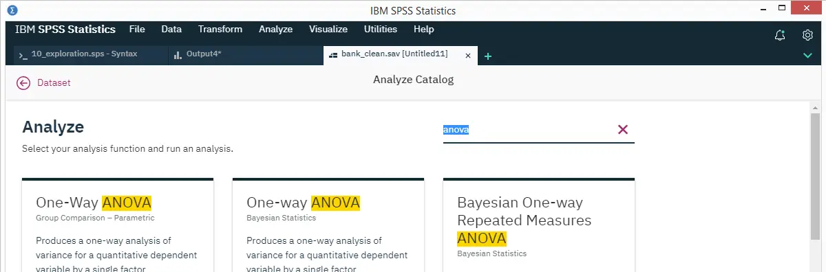
The search results lead me to the Oneway dialog but not GLM or MEANS. The problem here is that
- Oneway does not include partial eta squared, an effect size measure for ANOVA. We need to run our ANOVA from MEANS or GLM in order to get it;
- MEANS, however, does not offer Levene's test for homogeneity. We need either Oneway or GLM for that;
- If homogeneity doesn't hold, we may want to interpret the Welch statistic, only available in Oneway.
The real problem here is that a complete ANOVA can't be run from any single dialog or command in SPSS. Instead, we need to run a single analysis multiple times from different commands if we need all relevant output. And our search results don't even mention MEANS or GLM.
Ok, then let's search for a simpler analysis: the Kruskall-Wallis test.
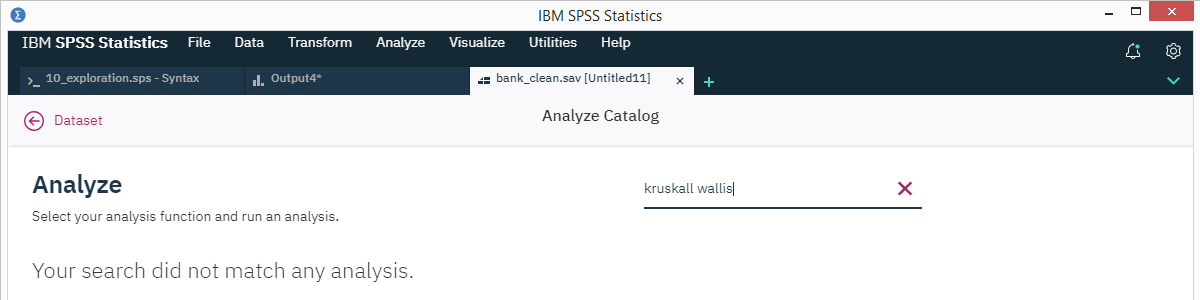
My search doesn't come up with anything at all. This is because I tested for a common misspelling of “Kruskal-Wallis test”. And the search function seems completely unable to handle it.
SPSS 26 - Conclusions
Summarizing this review, I think
SPSS’ new interface is worse than the old interface
in basically all regards:
- the visual layout -especially of the variable list and dialog tabs- is not as clear and simple as it used to be;
- essential functionality -such as pasting syntax and major analyses- are harder to find;
- most operations require more mouse clicks than they used to;
- many shortkeys no longer work -although a couple of new ones for navigating and closing tabs have been added.
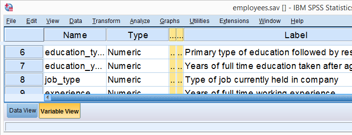 The nice and clear classic variable view
On top of that, the new interface is seriously incomplete. A handful of examples are that
- the View and Edit menus are missing;
- there's no Legacy Dialogs under Visualize;
- pivoting trays for rearranging pivot table dimensions aren't available;
- OMS information is unavailable from the output outline.
Some of those may be added to the new interface. But what about first finishing a product and then launching it?
In any case, I agree that SPSS urgently needs major improvements. This review hinted at a couple of those but there's tons more. Sadly, none of the things SPSS really needs was added to version 26. One thing SPSS did not really need, was a new interface.
If it ain't broken, don't fix it.
Thanks for reading.